

414
K. Example of a Cross Section Calculation
′
The four-dimensional δ-function then removes the integration over d
4 p
′ 2
leaving us only with an integration over the single δ-function δ(p −
′
M
2 ), in which p is understood to be replaced by k + p − k
′ . For details
of this last integration, see Bjorken and Drell (1964, p 114).
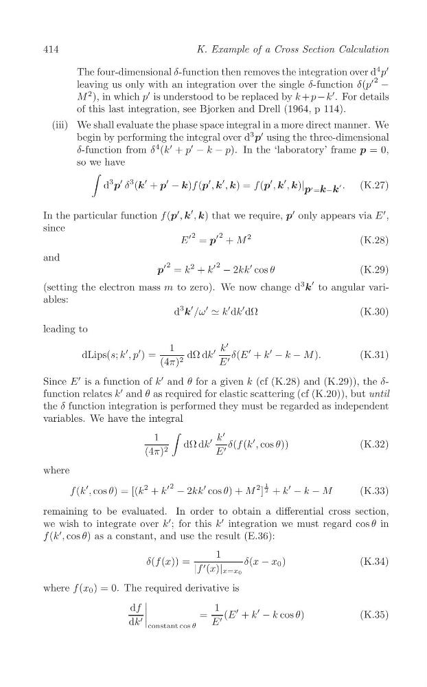
(iii) We shall evaluate the phase space integral in a more direct manner. We
d
3 ′
begin by performing the integral over p using the three-dimensional
′
δ-function from δ
4 (k
′ + p − k − p). In the ‘laboratory’ frame p = 0,
so we have
∫
′
′
′
d
3
p
′ δ
3 (k
′ + p − k)f (p , k
′ , k) = f (p , k
′ , k)| p ' =k−k
' . (K.27)
′
′
In the particular function f (p , k
′ , k) that we require, p only appears via E
′ ,
since
E
′ 2
′ 2
= p + M
2
(K.28)
and
′ 2
p = k
2 + k
′ 2 − 2kk
′ cos θ
(K.29)
(setting the electron mass m to zero). We now change d
3
k
′ to angular variables:
d
3
k
′ /ω
′
≃ k
′ dk
′ dΩ
(K.30)
leading to
dLips(s; k
′ , p
′ ) =
1 dΩ dk
′ k
′
δ(E
′ + k
′
− k − M ).
(K.31)
(4π) 2
E ′
Since E
′ is a function of k
′ and θ for a given k (cf (K.28) and (K.29)), the δfunction relates k
′ and θ as required for elastic scattering (cf (K.20)), but until
the δ function integration is performed they must be regarded as independent
variables. We have the integral
∫
1
k
′
dΩ dk
′
δ(f (k
′ , cos θ))
(K.32)
(4π) 2
E ′
where
2
f (k
′ , cos θ) = [(k
2 + k
′ 2 − 2kk
′ cos θ) + M
2 ]
1 + k
′
− k − M
(K.33)
remaining to be evaluated. In order to obtain a differential cross section,
we wish to integrate over k
′ ; for this k
′ integration we must regard cos θ in
f (k
′ , cos θ) as a constant, and use the result (E.36):
1
δ(f (x)) =
δ(x − x 0 )
(K.34)
|f ′ (x)| x=x0
where f (x 0 ) = 0. The required derivative is
df
=
1 (E
′ + k
′
− k cos θ)
(K.35)
dk ′
|
|
|
|
E ′
constant cos θ
K. Example of a Cross Section Calculation
′
The four-dimensional δ-function then removes the integration over d
4 p
′ 2
leaving us only with an integration over the single δ-function δ(p −
′
M
2 ), in which p is understood to be replaced by k + p − k
′ . For details
of this last integration, see Bjorken and Drell (1964, p 114).
(iii) We shall evaluate the phase space integral in a more direct manner. We
d
3 ′
begin by performing the integral over p using the three-dimensional
′
δ-function from δ
4 (k
′ + p − k − p). In the ‘laboratory’ frame p = 0,
so we have
∫
′
′
′
d
3
p
′ δ
3 (k
′ + p − k)f (p , k
′ , k) = f (p , k
′ , k)| p ' =k−k
' . (K.27)
′
′
In the particular function f (p , k
′ , k) that we require, p only appears via E
′ ,
since
E
′ 2
′ 2
= p + M
2
(K.28)
and
′ 2
p = k
2 + k
′ 2 − 2kk
′ cos θ
(K.29)
(setting the electron mass m to zero). We now change d
3
k
′ to angular variables:
d
3
k
′ /ω
′
≃ k
′ dk
′ dΩ
(K.30)
leading to
dLips(s; k
′ , p
′ ) =
1 dΩ dk
′ k
′
δ(E
′ + k
′
− k − M ).
(K.31)
(4π) 2
E ′
Since E
′ is a function of k
′ and θ for a given k (cf (K.28) and (K.29)), the δfunction relates k
′ and θ as required for elastic scattering (cf (K.20)), but until
the δ function integration is performed they must be regarded as independent
variables. We have the integral
∫
1
k
′
dΩ dk
′
δ(f (k
′ , cos θ))
(K.32)
(4π) 2
E ′
where
2
f (k
′ , cos θ) = [(k
2 + k
′ 2 − 2kk
′ cos θ) + M
2 ]
1 + k
′
− k − M
(K.33)
remaining to be evaluated. In order to obtain a differential cross section,
we wish to integrate over k
′ ; for this k
′ integration we must regard cos θ in
f (k
′ , cos θ) as a constant, and use the result (E.36):
1
δ(f (x)) =
δ(x − x 0 )
(K.34)
|f ′ (x)| x=x0
where f (x 0 ) = 0. The required derivative is
df
=
1 (E
′ + k
′
− k cos θ)
(K.35)
dk ′
|
|
|
|
E ′
constant cos θ