

21
1.3. Particle interactions in the Standard Model
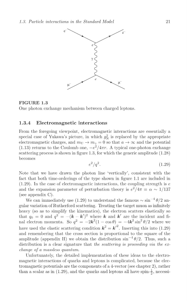
FIGURE 1.3
One photon exchange mechanism between charged leptons.
1.3.4 Electromagnetic interactions
From the foregoing viewpoint, electromagnetic interactions are essentially a
2
special case of Yukawa’s picture, in which g is replaced by the appropriate
N
electromagnetic charges, and m U → m γ = 0 so that a → ∞ and the potential
(1.13) returns to the Coulomb one, −e
2 /4πr. A typical one-photon exchange
scattering process is shown in figure 1.3, for which the generic amplitude (1.28)
becomes
e
2 /q
2 .
(1.29)
Note that we have drawn the photon line ‘vertically’, consistent with the
fact that both time-orderings of the type shown in figure 1.1 are included in
(1.29). In the case of electromagnetic interactions, the coupling strength is e
and the expansion parameter of perturbation theory is e
2 /4π ≡ α ∼ 1/137
(see appendix C).
We can immediately use (1.29) to understand the famous ∼ sin
−4 θ/2 angular variation of Rutherford scattering. Treating the target muon as infinitely
heavy (so as to simplify the kinematics), the electron scatters elastically so
2
that q 0 = 0 and q = −(k − k
′ )
2 where k and k
′ are the incident and fi2
nal electron momenta. So q = −2k
2 (1 − cos θ) = −4k
2 sin
2 θ/2 where we
k
′ 2
have used the elastic scattering condition k
2 =
. Inserting this into (1.29)
and remembering that the cross section is proportional to the square of the
amplitude (appendix H) we obtain the distribution sin
−4 θ/2. Thus, such a
distribution is a clear signature that the scattering is proceeding via the exchange of a massless quantum.
Unfortunately, the detailed implementation of these ideas to the electromagnetic interactions of quarks and leptons is complicated, because the electromagnetic potentials are the components of a 4-vector (see chapter 2), rather
than a scalar as in (1.29), and the quarks and leptons all have spin1 , necessi2
1.3. Particle interactions in the Standard Model
FIGURE 1.3
One photon exchange mechanism between charged leptons.
1.3.4 Electromagnetic interactions
From the foregoing viewpoint, electromagnetic interactions are essentially a
2
special case of Yukawa’s picture, in which g is replaced by the appropriate
N
electromagnetic charges, and m U → m γ = 0 so that a → ∞ and the potential
(1.13) returns to the Coulomb one, −e
2 /4πr. A typical one-photon exchange
scattering process is shown in figure 1.3, for which the generic amplitude (1.28)
becomes
e
2 /q
2 .
(1.29)
Note that we have drawn the photon line ‘vertically’, consistent with the
fact that both time-orderings of the type shown in figure 1.1 are included in
(1.29). In the case of electromagnetic interactions, the coupling strength is e
and the expansion parameter of perturbation theory is e
2 /4π ≡ α ∼ 1/137
(see appendix C).
We can immediately use (1.29) to understand the famous ∼ sin
−4 θ/2 angular variation of Rutherford scattering. Treating the target muon as infinitely
heavy (so as to simplify the kinematics), the electron scatters elastically so
2
that q 0 = 0 and q = −(k − k
′ )
2 where k and k
′ are the incident and fi2
nal electron momenta. So q = −2k
2 (1 − cos θ) = −4k
2 sin
2 θ/2 where we
k
′ 2
have used the elastic scattering condition k
2 =
. Inserting this into (1.29)
and remembering that the cross section is proportional to the square of the
amplitude (appendix H) we obtain the distribution sin
−4 θ/2. Thus, such a
distribution is a clear signature that the scattering is proceeding via the exchange of a massless quantum.
Unfortunately, the detailed implementation of these ideas to the electromagnetic interactions of quarks and leptons is complicated, because the electromagnetic potentials are the components of a 4-vector (see chapter 2), rather
than a scalar as in (1.29), and the quarks and leptons all have spin1 , necessi2