

20
1. The Particles and Forces of the Standard Model
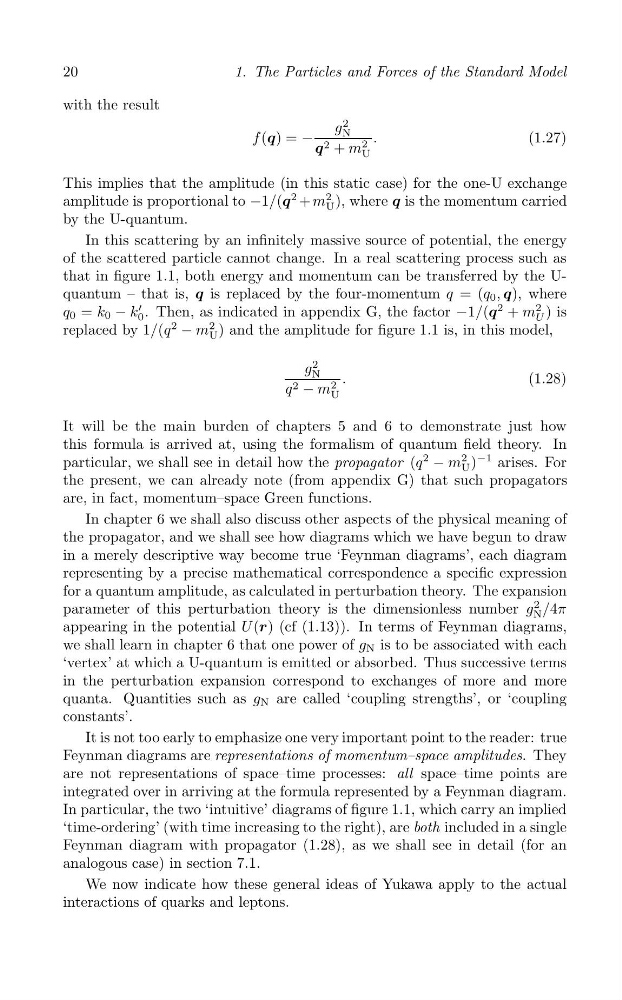
with the result
g
f (q) = −
2
N
.
(1.27)
q 2 + m 2
U
This implies that the amplitude (in this static case) for the one-U exchange
amplitude is proportional to −1/(q
2 + m
2
U ), where q is the momentum carried
by the U-quantum.
In this scattering by an infinitely massive source of potential, the energy
of the scattered particle cannot change. In a real scattering process such as
that in figure 1.1, both energy and momentum can be transferred by the Uquantum – that is, q is replaced by the four-momentum q = (q 0 , q), where
q 0 = k 0 − k 0
′ . Then, as indicated in appendix G, the factor −1/(q
2 + m
2
U ) is
replaced by 1/(q
2
− m
2
U ) and the amplitude for figure 1.1 is, in this model,
2
N
g
.
(1.28)
q 2 − m 2
U
It will be the main burden of chapters 5 and 6 to demonstrate just how
this formula is arrived at, using the formalism of quantum field theory. In
particular, we shall see in detail how the propagator (q
2
− m
2
U )
−1 arises. For
the present, we can already note (from appendix G) that such propagators
are, in fact, momentum–space Green functions.
In chapter 6 we shall also discuss other aspects of the physical meaning of
the propagator, and we shall see how diagrams which we have begun to draw
in a merely descriptive way become true ‘Feynman diagrams’, each diagram
representing by a precise mathematical correspondence a specific expression
for a quantum amplitude, as calculated in perturbation theory. The expansion
parameter of this perturbation theory is the dimensionless number g
2
N /4π
appearing in the potential U (r) (cf (1.13)). In terms of Feynman diagrams,
we shall learn in chapter 6 that one power of g N is to be associated with each
‘vertex’ at which a U-quantum is emitted or absorbed. Thus successive terms
in the perturbation expansion correspond to exchanges of more and more
quanta. Quantities such as g N are called ‘coupling strengths’, or ‘coupling
constants’.
It is not too early to emphasize one very important point to the reader: true
Feynman diagrams are representations of momentum–space amplitudes. They
are not representations of space–time processes: all space–time points are
integrated over in arriving at the formula represented by a Feynman diagram.
In particular, the two ‘intuitive’ diagrams of figure 1.1, which carry an implied
‘time-ordering’ (with time increasing to the right), are both included in a single
Feynman diagram with propagator (1.28), as we shall see in detail (for an
analogous case) in section 7.1.
We now indicate how these general ideas of Yukawa apply to the actual
interactions of quarks and leptons.
1. The Particles and Forces of the Standard Model
with the result
g
f (q) = −
2
N
.
(1.27)
q 2 + m 2
U
This implies that the amplitude (in this static case) for the one-U exchange
amplitude is proportional to −1/(q
2 + m
2
U ), where q is the momentum carried
by the U-quantum.
In this scattering by an infinitely massive source of potential, the energy
of the scattered particle cannot change. In a real scattering process such as
that in figure 1.1, both energy and momentum can be transferred by the Uquantum – that is, q is replaced by the four-momentum q = (q 0 , q), where
q 0 = k 0 − k 0
′ . Then, as indicated in appendix G, the factor −1/(q
2 + m
2
U ) is
replaced by 1/(q
2
− m
2
U ) and the amplitude for figure 1.1 is, in this model,
2
N
g
.
(1.28)
q 2 − m 2
U
It will be the main burden of chapters 5 and 6 to demonstrate just how
this formula is arrived at, using the formalism of quantum field theory. In
particular, we shall see in detail how the propagator (q
2
− m
2
U )
−1 arises. For
the present, we can already note (from appendix G) that such propagators
are, in fact, momentum–space Green functions.
In chapter 6 we shall also discuss other aspects of the physical meaning of
the propagator, and we shall see how diagrams which we have begun to draw
in a merely descriptive way become true ‘Feynman diagrams’, each diagram
representing by a precise mathematical correspondence a specific expression
for a quantum amplitude, as calculated in perturbation theory. The expansion
parameter of this perturbation theory is the dimensionless number g
2
N /4π
appearing in the potential U (r) (cf (1.13)). In terms of Feynman diagrams,
we shall learn in chapter 6 that one power of g N is to be associated with each
‘vertex’ at which a U-quantum is emitted or absorbed. Thus successive terms
in the perturbation expansion correspond to exchanges of more and more
quanta. Quantities such as g N are called ‘coupling strengths’, or ‘coupling
constants’.
It is not too early to emphasize one very important point to the reader: true
Feynman diagrams are representations of momentum–space amplitudes. They
are not representations of space–time processes: all space–time points are
integrated over in arriving at the formula represented by a Feynman diagram.
In particular, the two ‘intuitive’ diagrams of figure 1.1, which carry an implied
‘time-ordering’ (with time increasing to the right), are both included in a single
Feynman diagram with propagator (1.28), as we shall see in detail (for an
analogous case) in section 7.1.
We now indicate how these general ideas of Yukawa apply to the actual
interactions of quarks and leptons.