

320
10. Loops and Renormalization I: The ABC Theory
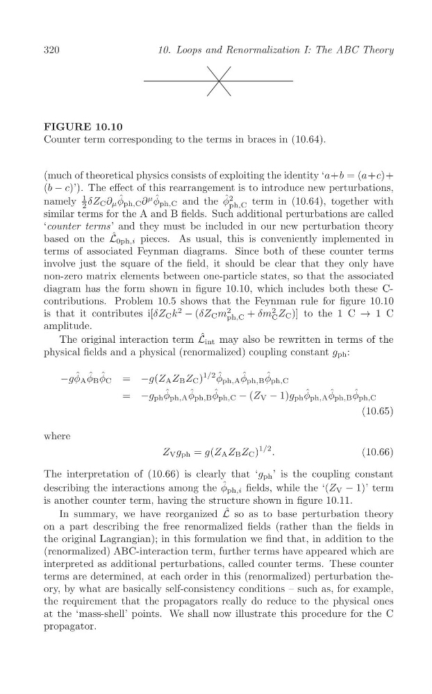
FIGURE 10.10
Counter term corresponding to the terms in braces in (10.64).
(much of theoretical physics consists of exploiting the identity ‘a+b = (a+c)+
(b − c)’). The effect of this rearrangement is to introduce new perturbations,
namely
1 δZ C ∂ μ φ ˆ ph,C ∂
μ φ ˆ ph,C and the φ ˆ2
term in (10.64), together with
2
ph,C
similar terms for the A and B fields. Such additional perturbations are called
‘counter terms’ and they must be included in our new perturbation theory
based on the L ˆ 0ph,i pieces. As usual, this is conveniently implemented in
terms of associated Feynman diagrams. Since both of these counter terms
involve just the square of the field, it should be clear that they only have
non-zero matrix elements between one-particle states, so that the associated
diagram has the form shown in figure 10.10, which includes both these Ccontributions. Problem 10.5 shows that the Feynman rule for figure 10.10
2
is that it contributes i[δZ C k
2
− (δZ C m ph,C + δm
2 Z C )] to the 1 C → 1 C
C
amplitude.
The original interaction term L ˆ int may also be rewritten in terms of the
physical fields and a physical (renormalized) coupling constant g ph :
−gφ ˆ A φ ˆ B φ ˆ C = −g(Z A Z B Z C )
1/2 φ ˆ ph,A φ ˆ ph,B φ ˆ ph,C
ˆ
ˆ
ˆ
ˆ
ˆ
ˆ
= −g ph φ ph,A φ ph,B φ ph,C − (Z V − 1)g ph φ ph,A φ ph,B φ ph,C
(10.65)
where
Z V g ph = g(Z A Z B Z C )
1/2 .
(10.66)
The interpretation of (10.66) is clearly that ‘g ph ’ is the coupling constant
describing the interactions among the φ ˆ ph,i fields, while the ‘(Z V − 1)’ term
is another counter term, having the structure shown in figure 10.11.
In summary, we have reorganized L ˆ so as to base perturbation theory
on a part describing the free renormalized fields (rather than the fields in
the original Lagrangian); in this formulation we find that, in addition to the
(renormalized) ABC-interaction term, further terms have appeared which are
interpreted as additional perturbations, called counter terms. These counter
terms are determined, at each order in this (renormalized) perturbation theory, by what are basically self-consistency conditions – such as, for example,
the requirement that the propagators really do reduce to the physical ones
at the ‘mass-shell’ points. We shall now illustrate this procedure for the C
propagator.
10. Loops and Renormalization I: The ABC Theory
FIGURE 10.10
Counter term corresponding to the terms in braces in (10.64).
(much of theoretical physics consists of exploiting the identity ‘a+b = (a+c)+
(b − c)’). The effect of this rearrangement is to introduce new perturbations,
namely
1 δZ C ∂ μ φ ˆ ph,C ∂
μ φ ˆ ph,C and the φ ˆ2
term in (10.64), together with
2
ph,C
similar terms for the A and B fields. Such additional perturbations are called
‘counter terms’ and they must be included in our new perturbation theory
based on the L ˆ 0ph,i pieces. As usual, this is conveniently implemented in
terms of associated Feynman diagrams. Since both of these counter terms
involve just the square of the field, it should be clear that they only have
non-zero matrix elements between one-particle states, so that the associated
diagram has the form shown in figure 10.10, which includes both these Ccontributions. Problem 10.5 shows that the Feynman rule for figure 10.10
2
is that it contributes i[δZ C k
2
− (δZ C m ph,C + δm
2 Z C )] to the 1 C → 1 C
C
amplitude.
The original interaction term L ˆ int may also be rewritten in terms of the
physical fields and a physical (renormalized) coupling constant g ph :
−gφ ˆ A φ ˆ B φ ˆ C = −g(Z A Z B Z C )
1/2 φ ˆ ph,A φ ˆ ph,B φ ˆ ph,C
ˆ
ˆ
ˆ
ˆ
ˆ
ˆ
= −g ph φ ph,A φ ph,B φ ph,C − (Z V − 1)g ph φ ph,A φ ph,B φ ph,C
(10.65)
where
Z V g ph = g(Z A Z B Z C )
1/2 .
(10.66)
The interpretation of (10.66) is clearly that ‘g ph ’ is the coupling constant
describing the interactions among the φ ˆ ph,i fields, while the ‘(Z V − 1)’ term
is another counter term, having the structure shown in figure 10.11.
In summary, we have reorganized L ˆ so as to base perturbation theory
on a part describing the free renormalized fields (rather than the fields in
the original Lagrangian); in this formulation we find that, in addition to the
(renormalized) ABC-interaction term, further terms have appeared which are
interpreted as additional perturbations, called counter terms. These counter
terms are determined, at each order in this (renormalized) perturbation theory, by what are basically self-consistency conditions – such as, for example,
the requirement that the propagators really do reduce to the physical ones
at the ‘mass-shell’ points. We shall now illustrate this procedure for the C
propagator.