

319
10.4. Bare and renormalized perturbation theory
in the original theory. Then the main effects, in some sense, would already be
included by the use of these (empirical) physical quantities, and corrections
would be ‘more plausibly’ small. This is indeed the main reason for the usefulness of such ‘effective’ parameters in the analogous case of condensed matter
physics. Actually, of course, in quantum field theory the corrections will be
just as infinite (if we send Λ to infinity) in this approach also, since whichever
way we set the calculation up, we shall get loops, which are divergent. All the
same, this kind of ‘reorganization’ does offer a more systematic approach to
renormalization.
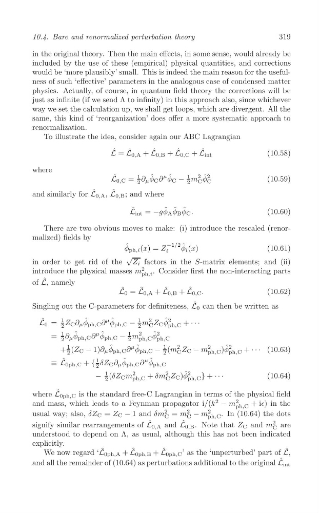
To illustrate the idea, consider again our ABC Lagrangian
L ˆ = L ˆ 0,A + L ˆ 0,B + L ˆ 0,C + L ˆ int
(10.58)
where
2
L ˆ 0,C =
1
φ ˆ C ∂
μ φ ˆ C −
1 m φ ˆ 2
(10.59)
2 ∂ μ
2 C C
and similarly for L ˆ 0,A , L ˆ 0,B ; and where
ˆ
ˆ ˆ ˆ
L int = −gφ A φ B φ C .
(10.60)
There are two obvious moves to make: (i) introduce the rescaled (renormalized) fields by
φ ˆ ph,i (x) = Z i
−1/2 φ ˆ i (x)
(10.61)
√
in order to get rid of the Z i factors in the S-matrix elements; and (ii)
2
introduce the physical masses m . Consider first the non-interacting parts
ph,i
of L ˆ , namely
L ˆ 0 = L ˆ 0,A + L ˆ 0,B + L ˆ 0,C .
(10.62)
Singling out the C-parameters for definiteness, L ˆ 0 can then be written as
ˆ
1
ˆ
2
φ ˆ 2
L 0 = 2 Z C ∂ μ φ ph,C ∂
μ φ ˆ ph,C − 2
1 m C Z C ph,C + · · ·
1
ˆ
2
φ ˆ 2
= ∂ μ φ ph,C ∂
μ φ ˆ ph,C −
1 m ph,C ph,C
1
ˆ
2
2
2
2
+ (Z C − 1)∂ μ φ ph,C ∂
μ φ ˆ ph,C −
1 (m C Z C − m
φ
2
· · · (10.63)
2
2
ph,C ) ˆ
ph,C +
ˆ
≡ ˆ
L 0ph,C + {
1 δZ C ∂ μ φ ph,C ∂
μ φ ˆ ph,C
2
1
2
− (δZ C m ph,C + δm C
2 Z C )φ ˆ 2
· · ·
(10.64)
2
ph,C } +
where L ˆ 0ph,C is the standard free-C Lagrangian in terms of the physical field
2
and mass, which leads to a Feynman propagator i/(k
2
− m ph,C + i∈) in the
2
2
usual way; also, δZ C = Z C − 1 and δm
2 = m C − m ph,C . In (10.64) the dots
C
2
signify similar rearrangements of L ˆ 0,A and L ˆ 0,B . Note that Z C and m are
C
understood to depend on Λ, as usual, although this has not been indicated
explicitly.
ˆ
We now regard ‘L 0ph,A + L ˆ 0ph,B + L ˆ 0ph,C ’ as the ‘unperturbed’ part of L ˆ ,
and all the remainder of (10.64) as perturbations additional to the original L ˆ int
10.4. Bare and renormalized perturbation theory
in the original theory. Then the main effects, in some sense, would already be
included by the use of these (empirical) physical quantities, and corrections
would be ‘more plausibly’ small. This is indeed the main reason for the usefulness of such ‘effective’ parameters in the analogous case of condensed matter
physics. Actually, of course, in quantum field theory the corrections will be
just as infinite (if we send Λ to infinity) in this approach also, since whichever
way we set the calculation up, we shall get loops, which are divergent. All the
same, this kind of ‘reorganization’ does offer a more systematic approach to
renormalization.
To illustrate the idea, consider again our ABC Lagrangian
L ˆ = L ˆ 0,A + L ˆ 0,B + L ˆ 0,C + L ˆ int
(10.58)
where
2
L ˆ 0,C =
1
φ ˆ C ∂
μ φ ˆ C −
1 m φ ˆ 2
(10.59)
2 ∂ μ
2 C C
and similarly for L ˆ 0,A , L ˆ 0,B ; and where
ˆ
ˆ ˆ ˆ
L int = −gφ A φ B φ C .
(10.60)
There are two obvious moves to make: (i) introduce the rescaled (renormalized) fields by
φ ˆ ph,i (x) = Z i
−1/2 φ ˆ i (x)
(10.61)
√
in order to get rid of the Z i factors in the S-matrix elements; and (ii)
2
introduce the physical masses m . Consider first the non-interacting parts
ph,i
of L ˆ , namely
L ˆ 0 = L ˆ 0,A + L ˆ 0,B + L ˆ 0,C .
(10.62)
Singling out the C-parameters for definiteness, L ˆ 0 can then be written as
ˆ
1
ˆ
2
φ ˆ 2
L 0 = 2 Z C ∂ μ φ ph,C ∂
μ φ ˆ ph,C − 2
1 m C Z C ph,C + · · ·
1
ˆ
2
φ ˆ 2
= ∂ μ φ ph,C ∂
μ φ ˆ ph,C −
1 m ph,C ph,C
1
ˆ
2
2
2
2
+ (Z C − 1)∂ μ φ ph,C ∂
μ φ ˆ ph,C −
1 (m C Z C − m
φ
2
· · · (10.63)
2
2
ph,C ) ˆ
ph,C +
ˆ
≡ ˆ
L 0ph,C + {
1 δZ C ∂ μ φ ph,C ∂
μ φ ˆ ph,C
2
1
2
− (δZ C m ph,C + δm C
2 Z C )φ ˆ 2
· · ·
(10.64)
2
ph,C } +
where L ˆ 0ph,C is the standard free-C Lagrangian in terms of the physical field
2
and mass, which leads to a Feynman propagator i/(k
2
− m ph,C + i∈) in the
2
2
usual way; also, δZ C = Z C − 1 and δm
2 = m C − m ph,C . In (10.64) the dots
C
2
signify similar rearrangements of L ˆ 0,A and L ˆ 0,B . Note that Z C and m are
C
understood to depend on Λ, as usual, although this has not been indicated
explicitly.
ˆ
We now regard ‘L 0ph,A + L ˆ 0ph,B + L ˆ 0ph,C ’ as the ‘unperturbed’ part of L ˆ ,
and all the remainder of (10.64) as perturbations additional to the original L ˆ int