

316
10. Loops and Renormalization I: The ABC Theory
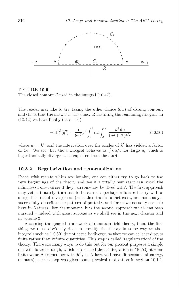
FIGURE 10.9
The closed contour C used in the integral (10.47).
The reader may like to try taking the other choice (C − ) of closing contour,
and check that the answer is the same. Reinstating the remaining integrals in
(10.42) we have finally (as ∈ → 0)
∫
∫
i
1
∞
u
2 du
2
−iΠ
[2] (q
2 ) =
g
dx
(10.50)
C
8π 2
(u 2 + Δ) 3/2
0
0
where u = |k
′
| and the integration over the angles of k
′ has yielded a factor
∫
of 4π. We see that the u-integral behaves as du/u for large u, which is
logarithmically divergent, as expected from the start.
10.3.2 Regularization and renormalization
Faced with results which are infinite, one can either try to go back to the
very beginnings of the theory and see if a totally new start can avoid the
infinities or one can see if they can somehow be ‘lived with’. The first approach
may yet, ultimately, turn out to be correct: perhaps a future theory will be
altogether free of divergences (such theories do in fact exist, but none as yet
successfully describes the pattern of particles and forces we actually seem to
have in Nature). For the moment, it is the second approach which has been
pursued – indeed with great success as we shall see in the next chapter and
in volume 2.
Accepting the general framework of quantum field theory, then, the first
thing we must obviously do is to modify the theory in some way so that
integrals such as (10.50) do not actually diverge, so that we can at least discuss
finite rather than infinite quantities. This step is called ‘regularization’ of the
theory. There are many ways to do this but for our present purposes a simple
one will do well enough, which is to cut off the u-integration in (10.50) at some
finite value Λ (remember u is |k
′ |, so Λ here will have dimensions of energy,
or mass); such a step was given some physical motivation in section 10.1.1.
10. Loops and Renormalization I: The ABC Theory
FIGURE 10.9
The closed contour C used in the integral (10.47).
The reader may like to try taking the other choice (C − ) of closing contour,
and check that the answer is the same. Reinstating the remaining integrals in
(10.42) we have finally (as ∈ → 0)
∫
∫
i
1
∞
u
2 du
2
−iΠ
[2] (q
2 ) =
g
dx
(10.50)
C
8π 2
(u 2 + Δ) 3/2
0
0
where u = |k
′
| and the integration over the angles of k
′ has yielded a factor
∫
of 4π. We see that the u-integral behaves as du/u for large u, which is
logarithmically divergent, as expected from the start.
10.3.2 Regularization and renormalization
Faced with results which are infinite, one can either try to go back to the
very beginnings of the theory and see if a totally new start can avoid the
infinities or one can see if they can somehow be ‘lived with’. The first approach
may yet, ultimately, turn out to be correct: perhaps a future theory will be
altogether free of divergences (such theories do in fact exist, but none as yet
successfully describes the pattern of particles and forces we actually seem to
have in Nature). For the moment, it is the second approach which has been
pursued – indeed with great success as we shall see in the next chapter and
in volume 2.
Accepting the general framework of quantum field theory, then, the first
thing we must obviously do is to modify the theory in some way so that
integrals such as (10.50) do not actually diverge, so that we can at least discuss
finite rather than infinite quantities. This step is called ‘regularization’ of the
theory. There are many ways to do this but for our present purposes a simple
one will do well enough, which is to cut off the u-integration in (10.50) at some
finite value Λ (remember u is |k
′ |, so Λ here will have dimensions of energy,
or mass); such a step was given some physical motivation in section 10.1.1.