

315
10.3. Dealing with the bad news: a simple example
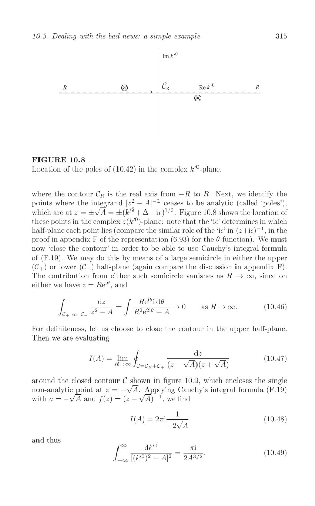
FIGURE 10.8
Location of the poles of (10.42) in the complex k
′0 -plane.
where the contour C R is the real axis from −R to R. Next, we identify the
points where the integrand [z
2
− A]
−1 ceases to be analytic (called ‘poles’),
√
which are at z = ± A = ±(k
′2 + Δ− i∈)
1/2 . Figure 10.8 shows the location of
these points in the complex z(k
′0 )-plane: note that the ‘i∈’ determines in which
half-plane each point lies (compare the similar role of the ‘i∈’ in (z+i∈)
−1 , in the
proof in appendix F of the representation (6.93) for the θ-function). We must
now ‘close the contour’ in order to be able to use Cauchy’s integral formula
of (F.19). We may do this by means of a large semicircle in either the upper
(C + ) or lower (C − ) half-plane (again compare the discussion in appendix F).
The contribution from either such semicircle vanishes as R → ∞, since on
either we have z = Re
iθ , and
∫
∫
dz
Re
iθ i dθ
=
→ 0
as R → ∞.
(10.46)
R 2 e 2iθ − A
z 2 − A
C+ or C−
For definiteness, let us choose to close the contour in the upper half-plane.
Then we are evaluating
∮
dz
I(A) = lim
√
√
(10.47)
R→∞ C=CR+C+ (z − A)(z + A)
around the closed contour C shown in figure 10.9, which encloses the single
√
non-analytic point at z = − A. Applying Cauchy’s integral formula (F.19)
√
√
with a = − A and f (z) = (z − A)
−1 , we find
1
I(A) = 2πi √
(10.48)
−2 A
and thus
∫ ∞
dk
′0
πi
=
.
(10.49)
[(k ′0 ) 2 − A] 2
2A 3/2
−∞
10.3. Dealing with the bad news: a simple example
FIGURE 10.8
Location of the poles of (10.42) in the complex k
′0 -plane.
where the contour C R is the real axis from −R to R. Next, we identify the
points where the integrand [z
2
− A]
−1 ceases to be analytic (called ‘poles’),
√
which are at z = ± A = ±(k
′2 + Δ− i∈)
1/2 . Figure 10.8 shows the location of
these points in the complex z(k
′0 )-plane: note that the ‘i∈’ determines in which
half-plane each point lies (compare the similar role of the ‘i∈’ in (z+i∈)
−1 , in the
proof in appendix F of the representation (6.93) for the θ-function). We must
now ‘close the contour’ in order to be able to use Cauchy’s integral formula
of (F.19). We may do this by means of a large semicircle in either the upper
(C + ) or lower (C − ) half-plane (again compare the discussion in appendix F).
The contribution from either such semicircle vanishes as R → ∞, since on
either we have z = Re
iθ , and
∫
∫
dz
Re
iθ i dθ
=
→ 0
as R → ∞.
(10.46)
R 2 e 2iθ − A
z 2 − A
C+ or C−
For definiteness, let us choose to close the contour in the upper half-plane.
Then we are evaluating
∮
dz
I(A) = lim
√
√
(10.47)
R→∞ C=CR+C+ (z − A)(z + A)
around the closed contour C shown in figure 10.9, which encloses the single
√
non-analytic point at z = − A. Applying Cauchy’s integral formula (F.19)
√
√
with a = − A and f (z) = (z − A)
−1 , we find
1
I(A) = 2πi √
(10.48)
−2 A
and thus
∫ ∞
dk
′0
πi
=
.
(10.49)
[(k ′0 ) 2 − A] 2
2A 3/2
−∞