

312
10. Loops and Renormalization I: The ABC Theory
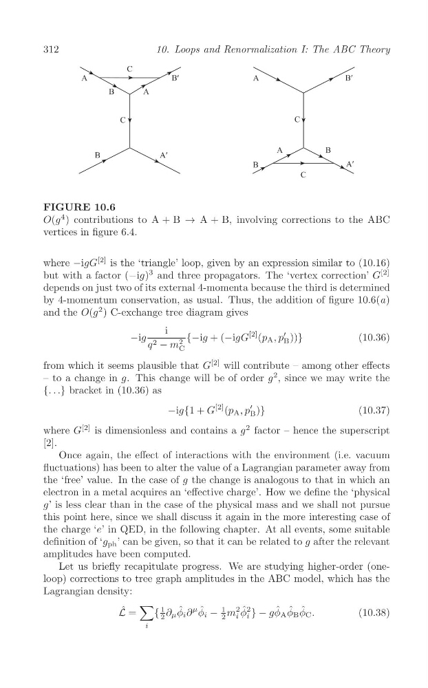
FIGURE 10.6
O(g
4 ) contributions to A + B → A + B, involving corrections to the ABC
vertices in figure 6.4.
where −igG
[2] is the ‘triangle’ loop, given by an expression similar to (10.16)
but with a factor (−ig)
3 and three propagators. The ‘vertex correction’ G
[2]
depends on just two of its external 4-momenta because the third is determined
by 4-momentum conservation, as usual. Thus, the addition of figure 10.6(a)
and the O(g
2 ) C-exchange tree diagram gives
i
−ig
{−ig + (−igG
[2] (p A , p B
′ ))}
(10.36)
2
q 2 − m C
from which it seems plausible that G
[2] will contribute – among other effects
– to a change in g. This change will be of order g
2 , since we may write the
{. . .} bracket in (10.36) as
−ig{1 + G
[2] (p A , p
′
B )}
(10.37)
2
where G
[2] is dimensionless and contains a g factor – hence the superscript
[2].
Once again, the effect of interactions with the environment (i.e. vacuum
fluctuations) has been to alter the value of a Lagrangian parameter away from
the ‘free’ value. In the case of g the change is analogous to that in which an
electron in a metal acquires an ‘effective charge’. How we define the ‘physical
g’ is less clear than in the case of the physical mass and we shall not pursue
this point here, since we shall discuss it again in the more interesting case of
the charge ‘e’ in QED, in the following chapter. At all events, some suitable
definition of ‘g ph ’ can be given, so that it can be related to g after the relevant
amplitudes have been computed.
Let us briefly recapitulate progress. We are studying higher-order (oneloop) corrections to tree graph amplitudes in the ABC model, which has the
Lagrangian density:
∑
L ˆ =
{
1 ∂ μ φ ˆ i ∂
μ φ ˆ i −
1 m
2 φ ˆ 2
i } − gφ ˆ A φ ˆ B φ ˆ C .
(10.38)
2
2 i
i
10. Loops and Renormalization I: The ABC Theory
FIGURE 10.6
O(g
4 ) contributions to A + B → A + B, involving corrections to the ABC
vertices in figure 6.4.
where −igG
[2] is the ‘triangle’ loop, given by an expression similar to (10.16)
but with a factor (−ig)
3 and three propagators. The ‘vertex correction’ G
[2]
depends on just two of its external 4-momenta because the third is determined
by 4-momentum conservation, as usual. Thus, the addition of figure 10.6(a)
and the O(g
2 ) C-exchange tree diagram gives
i
−ig
{−ig + (−igG
[2] (p A , p B
′ ))}
(10.36)
2
q 2 − m C
from which it seems plausible that G
[2] will contribute – among other effects
– to a change in g. This change will be of order g
2 , since we may write the
{. . .} bracket in (10.36) as
−ig{1 + G
[2] (p A , p
′
B )}
(10.37)
2
where G
[2] is dimensionless and contains a g factor – hence the superscript
[2].
Once again, the effect of interactions with the environment (i.e. vacuum
fluctuations) has been to alter the value of a Lagrangian parameter away from
the ‘free’ value. In the case of g the change is analogous to that in which an
electron in a metal acquires an ‘effective charge’. How we define the ‘physical
g’ is less clear than in the case of the physical mass and we shall not pursue
this point here, since we shall discuss it again in the more interesting case of
the charge ‘e’ in QED, in the following chapter. At all events, some suitable
definition of ‘g ph ’ can be given, so that it can be related to g after the relevant
amplitudes have been computed.
Let us briefly recapitulate progress. We are studying higher-order (oneloop) corrections to tree graph amplitudes in the ABC model, which has the
Lagrangian density:
∑
L ˆ =
{
1 ∂ μ φ ˆ i ∂
μ φ ˆ i −
1 m
2 φ ˆ 2
i } − gφ ˆ A φ ˆ B φ ˆ C .
(10.38)
2
2 i
i