

311
10.2. The vertex correction
(0)
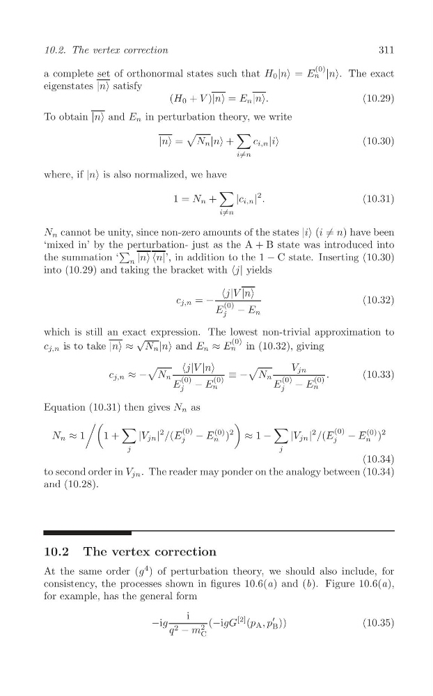
a complete set of orthonormal states such that H 0 |n> = E n |n>. The exact
eigenstates |n> satisfy
(H 0 + V )|n> = E n |n>.
(10.29)
To obtain |n> and E n in perturbation theory, we write
∑
√
|n> = N n |n> +
c i,n |i>
(10.30)
i/ =n
where, if |n> is also normalized, we have
∑
2
1 = N n +
|c i,n | .
(10.31)
i/ =n
N n cannot be unity, since non-zero amounts of the states |i> (i / = n) have been
‘mixed in’ by the perturbation- just as the A + B state was introduced into
∑
the summation ‘
|n>
into (10.29) and taking the bracket with
c j,n = − (0)
(10.32)
E − E n
j
which is still an exact expression. The lowest non-trivial approximation to
√
(0)
c j,n is to take |n> ≈ N n |n> and E n ≈ E n in (10.32), giving
√
√
V jn
c j,n ≈ − N n
≡ − N n
.
(10.33)
(0)
(0)
(0)
(0)
E − E n
E − E n
j
j
Equation (10.31) then gives N n as
/(
)
∑
∑
N n ≈ 1
1 +
|V jn |
2 /(E j
(0) − E
(0) )
2
≈ 1 −
|V jn |
2 /(E
(0) − E n
(0) )
2
n
j
j
j
(10.34)
to second order in V jn . The reader may ponder on the analogy between (10.34)
and (10.28).
10.2 The vertex correction
At the same order (g
4 ) of perturbation theory, we should also include, for
consistency, the processes shown in figures 10.6(a) and (b). Figure 10.6(a),
for example, has the general form
i
(−igG
[2] (p A , p
′
−ig
B ))
(10.35)
2
q 2 − m C
10.2. The vertex correction
(0)
a complete set of orthonormal states such that H 0 |n> = E n |n>. The exact
eigenstates |n> satisfy
(H 0 + V )|n> = E n |n>.
(10.29)
To obtain |n> and E n in perturbation theory, we write
∑
√
|n> = N n |n> +
c i,n |i>
(10.30)
i/ =n
where, if |n> is also normalized, we have
∑
2
1 = N n +
|c i,n | .
(10.31)
i/ =n
N n cannot be unity, since non-zero amounts of the states |i> (i / = n) have been
‘mixed in’ by the perturbation- just as the A + B state was introduced into
∑
the summation ‘
|n>
into (10.29) and taking the bracket with
c j,n = − (0)
(10.32)
E − E n
j
which is still an exact expression. The lowest non-trivial approximation to
√
(0)
c j,n is to take |n> ≈ N n |n> and E n ≈ E n in (10.32), giving
√
√
V jn
c j,n ≈ − N n
≡ − N n
.
(10.33)
(0)
(0)
(0)
(0)
E − E n
E − E n
j
j
Equation (10.31) then gives N n as
/(
)
∑
∑
N n ≈ 1
1 +
|V jn |
2 /(E j
(0) − E
(0) )
2
≈ 1 −
|V jn |
2 /(E
(0) − E n
(0) )
2
n
j
j
j
(10.34)
to second order in V jn . The reader may ponder on the analogy between (10.34)
and (10.28).
10.2 The vertex correction
At the same order (g
4 ) of perturbation theory, we should also include, for
consistency, the processes shown in figures 10.6(a) and (b). Figure 10.6(a),
for example, has the general form
i
(−igG
[2] (p A , p
′
−ig
B ))
(10.35)
2
q 2 − m C