

310
10. Loops and Renormalization I: The ABC Theory
where the states |n> are now the exact eigenstates of the full Hamiltonian. The
crucial difference between (10.23) and (10.25) is that in (10.25), multi-particle
states can appear in the states |n>. For example, the state |A, B> consisting
of an A particle and a B particle will enter, because the interaction couples
this state to the 1-C states created and destroyed in φ ˆ C : indeed, just such an
[2]
A+B state is present in Π ! This means that, whereas in the free case the
C
‘content’ of the state <0|φ ˆ C (x) was fully exhausted by the 1 − C state |C, k>
(in the sense that all overlaps with other states |n> were zero), this is not so
in the interacting case. The ‘content’ of <Ω|φ ˆ C (x) is not fully exhausted by
the state |C, k>: rather, it has overlaps with many other states. Now the sum
∑
total of all these overlaps (in the sense of ‘
|n>
it seems clear that the ‘strength’ of the single matrix element <Ω|φ ˆ C (x)|C, k>
in the interacting case cannot be the same as the free case (where the single
state exhausted the completeness sum). However, we expect it to be true that
<Ω|φ ˆ C (x)|C, k> is still basically the wavefunction for the C-particle. Hence we
shall write
√
−ik·x
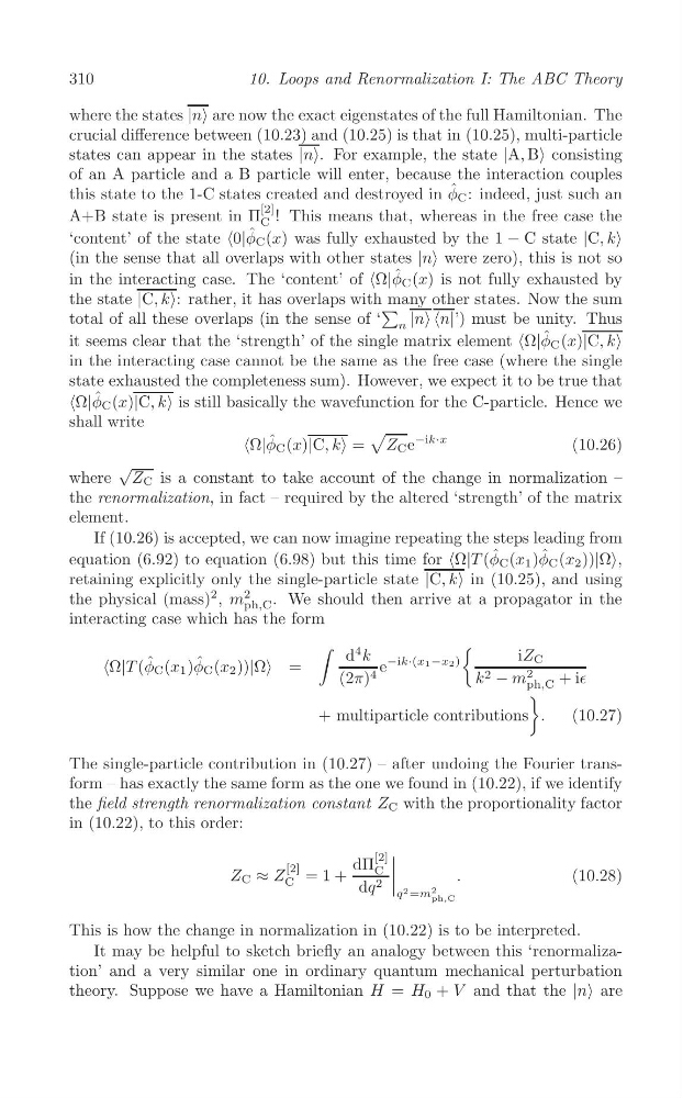
<Ω|φ ˆ C (x)|C, k> = Z C e
(10.26)
√
where Z C is a constant to take account of the change in normalization –
the renormalization, in fact – required by the altered ‘strength’ of the matrix
element.
If (10.26) is accepted, we can now imagine repeating the steps leading from
equation (6.92) to equation (6.98) but this time for <Ω|T (φ ˆ C (x 1 )φ ˆ C (x 2 ))|Ω>,
retaining explicitly only the single-particle state |C, k> in (10.25), and using
2
the physical (mass)
2 , m
We should then arrive at a propagator in the
ph,C .
interacting case which has the form
∫
(
d
4 k
iZ C
−ik·(x1−x2)
<Ω|T (φ ˆ C (x 1 )φ ˆ C (x 2 ))|Ω> =
e
2
(2π) 4
k 2 − m ph,C + i∈
)
+ multiparticle contributions .
(10.27)
The single-particle contribution in (10.27) – after undoing the Fourier transform – has exactly the same form as the one we found in (10.22), if we identify
the field strength renormalization constant Z C with the proportionality factor
in (10.22), to this order:
[2]
dΠ
[2]
C
Z C ≈ Z = 1 +
.
(10.28)
C
|
|
|
|
dq 2
2
q 2 =m ph,C
This is how the change in normalization in (10.22) is to be interpreted.
It may be helpful to sketch briefly an analogy between this ‘renormalization’ and a very similar one in ordinary quantum mechanical perturbation
theory. Suppose we have a Hamiltonian H = H 0 + V and that the |n> are
10. Loops and Renormalization I: The ABC Theory
where the states |n> are now the exact eigenstates of the full Hamiltonian. The
crucial difference between (10.23) and (10.25) is that in (10.25), multi-particle
states can appear in the states |n>. For example, the state |A, B> consisting
of an A particle and a B particle will enter, because the interaction couples
this state to the 1-C states created and destroyed in φ ˆ C : indeed, just such an
[2]
A+B state is present in Π ! This means that, whereas in the free case the
C
‘content’ of the state <0|φ ˆ C (x) was fully exhausted by the 1 − C state |C, k>
(in the sense that all overlaps with other states |n> were zero), this is not so
in the interacting case. The ‘content’ of <Ω|φ ˆ C (x) is not fully exhausted by
the state |C, k>: rather, it has overlaps with many other states. Now the sum
∑
total of all these overlaps (in the sense of ‘
|n>
it seems clear that the ‘strength’ of the single matrix element <Ω|φ ˆ C (x)|C, k>
in the interacting case cannot be the same as the free case (where the single
state exhausted the completeness sum). However, we expect it to be true that
<Ω|φ ˆ C (x)|C, k> is still basically the wavefunction for the C-particle. Hence we
shall write
√
−ik·x
<Ω|φ ˆ C (x)|C, k> = Z C e
(10.26)
√
where Z C is a constant to take account of the change in normalization –
the renormalization, in fact – required by the altered ‘strength’ of the matrix
element.
If (10.26) is accepted, we can now imagine repeating the steps leading from
equation (6.92) to equation (6.98) but this time for <Ω|T (φ ˆ C (x 1 )φ ˆ C (x 2 ))|Ω>,
retaining explicitly only the single-particle state |C, k> in (10.25), and using
2
the physical (mass)
2 , m
We should then arrive at a propagator in the
ph,C .
interacting case which has the form
∫
(
d
4 k
iZ C
−ik·(x1−x2)
<Ω|T (φ ˆ C (x 1 )φ ˆ C (x 2 ))|Ω> =
e
2
(2π) 4
k 2 − m ph,C + i∈
)
+ multiparticle contributions .
(10.27)
The single-particle contribution in (10.27) – after undoing the Fourier transform – has exactly the same form as the one we found in (10.22), if we identify
the field strength renormalization constant Z C with the proportionality factor
in (10.22), to this order:
[2]
dΠ
[2]
C
Z C ≈ Z = 1 +
.
(10.28)
C
|
|
|
|
dq 2
2
q 2 =m ph,C
This is how the change in normalization in (10.22) is to be interpreted.
It may be helpful to sketch briefly an analogy between this ‘renormalization’ and a very similar one in ordinary quantum mechanical perturbation
theory. Suppose we have a Hamiltonian H = H 0 + V and that the |n> are