

306
10. Loops and Renormalization I: The ABC Theory
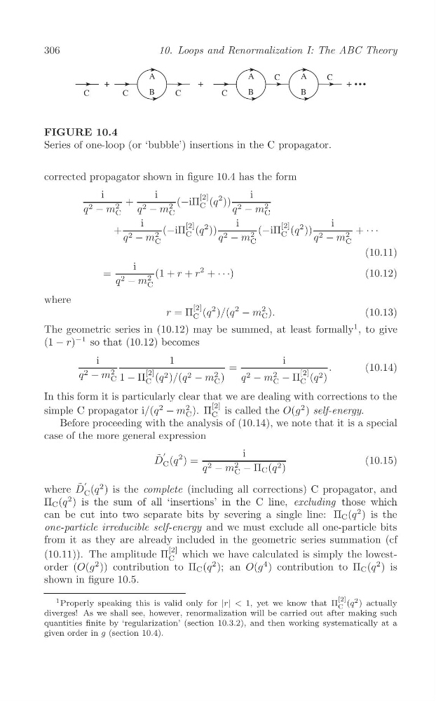
FIGURE 10.4
Series of one-loop (or ‘bubble’) insertions in the C propagator.
corrected propagator shown in figure 10.4 has the form
i
i
i
+
(−iΠ
[2] (q
2 ))
2
2
C
2
q 2 − m
q 2 − m
q 2 − m
C
C
C
i
i
i
[2]
[2]
+
(−iΠ (q
2 ))
(−iΠ (q
2 ))
+ · · ·
2
C
2
C
2
q 2 − m
q 2 − m
q 2 − m
C
C
C
(10.11)
i
2
=
(1 + r + r + · · ·)
(10.12)
2
q 2 − m C
where
[2]
2
r = Π (q
2 )/(q
2
− m C ).
(10.13)
C
The geometric series in (10.12) may be summed, at least formally
1 , to give
(1 − r)
−1 so that (10.12) becomes
i
1
i
=
.
(10.14)
q 2 − m 2
[2]
2
2
[2]
C 1 − Π (q 2 )/(q 2 − m )
q 2 − m − Π (q 2 )
C
C
C
C
In this form it is particularly clear that we are dealing with corrections to the
2
simple C propagator i/(q
2
− m ). Π
[2] is called the O(g
2 ) self-energy.
C
C
Before proceeding with the analysis of (10.14), we note that it is a special
case of the more general expression
'
i
D ˜
C (q
2 ) =
(10.15)
2
q 2 − m − Π C (q 2 )
C
where D ˜
' (q
2 ) is the complete (including all corrections) C propagator, and
C
Π C (q
2 ) is the sum of all ‘insertions’ in the C line, excluding those which
can be cut into two separate bits by severing a single line: Π C (q
2 ) is the
one-particle irreducible self-energy and we must exclude all one-particle bits
from it as they are already included in the geometric series summation (cf
[2]
(10.11)). The amplitude Π which we have calculated is simply the lowestC
order (O(g
2 )) contribution to Π C (q
2 ); an O(g
4 ) contribution to Π C (q
2 ) is
shown in figure 10.5.
[2]
1 Properly speaking this is valid only for |r| < 1, yet we know that Π (q 2 ) actually
C
diverges! As we shall see, however, renormalization will be carried out after making such
quantities finite by ‘regularization’ (section 10.3.2), and then working systematically at a
given order in g (section 10.4).
10. Loops and Renormalization I: The ABC Theory
FIGURE 10.4
Series of one-loop (or ‘bubble’) insertions in the C propagator.
corrected propagator shown in figure 10.4 has the form
i
i
i
+
(−iΠ
[2] (q
2 ))
2
2
C
2
q 2 − m
q 2 − m
q 2 − m
C
C
C
i
i
i
[2]
[2]
+
(−iΠ (q
2 ))
(−iΠ (q
2 ))
+ · · ·
2
C
2
C
2
q 2 − m
q 2 − m
q 2 − m
C
C
C
(10.11)
i
2
=
(1 + r + r + · · ·)
(10.12)
2
q 2 − m C
where
[2]
2
r = Π (q
2 )/(q
2
− m C ).
(10.13)
C
The geometric series in (10.12) may be summed, at least formally
1 , to give
(1 − r)
−1 so that (10.12) becomes
i
1
i
=
.
(10.14)
q 2 − m 2
[2]
2
2
[2]
C 1 − Π (q 2 )/(q 2 − m )
q 2 − m − Π (q 2 )
C
C
C
C
In this form it is particularly clear that we are dealing with corrections to the
2
simple C propagator i/(q
2
− m ). Π
[2] is called the O(g
2 ) self-energy.
C
C
Before proceeding with the analysis of (10.14), we note that it is a special
case of the more general expression
'
i
D ˜
C (q
2 ) =
(10.15)
2
q 2 − m − Π C (q 2 )
C
where D ˜
' (q
2 ) is the complete (including all corrections) C propagator, and
C
Π C (q
2 ) is the sum of all ‘insertions’ in the C line, excluding those which
can be cut into two separate bits by severing a single line: Π C (q
2 ) is the
one-particle irreducible self-energy and we must exclude all one-particle bits
from it as they are already included in the geometric series summation (cf
[2]
(10.11)). The amplitude Π which we have calculated is simply the lowestC
order (O(g
2 )) contribution to Π C (q
2 ); an O(g
4 ) contribution to Π C (q
2 ) is
shown in figure 10.5.
[2]
1 Properly speaking this is valid only for |r| < 1, yet we know that Π (q 2 ) actually
C
diverges! As we shall see, however, renormalization will be carried out after making such
quantities finite by ‘regularization’ (section 10.3.2), and then working systematically at a
given order in g (section 10.4).