

305
10.1. The propagator correction in ABC theory
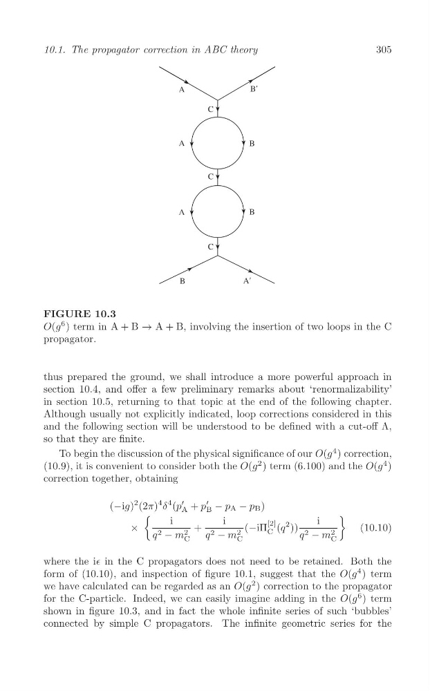
FIGURE 10.3
O(g
6 ) term in A + B → A + B, involving the insertion of two loops in the C
propagator.
thus prepared the ground, we shall introduce a more powerful approach in
section 10.4, and offer a few preliminary remarks about ‘renormalizability’
in section 10.5, returning to that topic at the end of the following chapter.
Although usually not explicitly indicated, loop corrections considered in this
and the following section will be understood to be defined with a cut-off Λ,
so that they are finite.
To begin the discussion of the physical significance of our O(g
4 ) correction,
(10.9), it is convenient to consider both the O(g
2 ) term (6.100) and the O(g
4 )
correction together, obtaining
′
′
(−ig)
2 (2π)
4 δ
4 (p A + p B − p A − p B )
(
)
i
i
i
×
+
(−iΠ
[2] (q
2 ))
(10.10)
2
2
C
2
q 2 − m
q 2 − m
q 2 − m
C
C
C
where the i∈ in the C propagators does not need to be retained. Both the
form of (10.10), and inspection of figure 10.1, suggest that the O(g
4 ) term
we have calculated can be regarded as an O(g
2 ) correction to the propagator
for the C-particle. Indeed, we can easily imagine adding in the O(g
6 ) term
shown in figure 10.3, and in fact the whole infinite series of such ‘bubbles’
connected by simple C propagators. The infinite geometric series for the
10.1. The propagator correction in ABC theory
FIGURE 10.3
O(g
6 ) term in A + B → A + B, involving the insertion of two loops in the C
propagator.
thus prepared the ground, we shall introduce a more powerful approach in
section 10.4, and offer a few preliminary remarks about ‘renormalizability’
in section 10.5, returning to that topic at the end of the following chapter.
Although usually not explicitly indicated, loop corrections considered in this
and the following section will be understood to be defined with a cut-off Λ,
so that they are finite.
To begin the discussion of the physical significance of our O(g
4 ) correction,
(10.9), it is convenient to consider both the O(g
2 ) term (6.100) and the O(g
4 )
correction together, obtaining
′
′
(−ig)
2 (2π)
4 δ
4 (p A + p B − p A − p B )
(
)
i
i
i
×
+
(−iΠ
[2] (q
2 ))
(10.10)
2
2
C
2
q 2 − m
q 2 − m
q 2 − m
C
C
C
where the i∈ in the C propagators does not need to be retained. Both the
form of (10.10), and inspection of figure 10.1, suggest that the O(g
4 ) term
we have calculated can be regarded as an O(g
2 ) correction to the propagator
for the C-particle. Indeed, we can easily imagine adding in the O(g
6 ) term
shown in figure 10.3, and in fact the whole infinite series of such ‘bubbles’
connected by simple C propagators. The infinite geometric series for the