

253
8.6. Electron Compton scattering
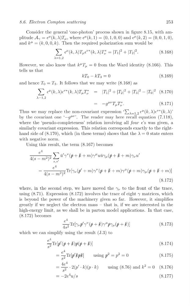
Consider the general ‘one-photon’ process shown in figure 8.15, with amplitude A γ = ∈
μ (k, λ)T μ , where ∈
μ (k, 1) = (0, 1, 0, 0) and ∈
μ (k, 2) = (0, 0, 1, 0),
and k
μ = (k, 0, 0, k). Then the required polarization sum would be
∑
∗
2
2
∈
μ (k, λ)T μ ∈
ν∗ (k, λ)T = |T 1 | + |T 2 | .
(8.168)
ν
λ=1,2
However, we also know that k
μ T μ = 0 from the Ward identity (8.166). This
tells us that
kT 0 − kT 3 = 0
(8.169)
and hence T 0 = T 3 . It follows that we may write (8.168) as
∑
∗
2
2
2
∈
μ (k, λ)∈
ν∗ (k, λ)T μ T
= |T 1 | + |T 2 | + |T 3 |
2
− |T 0 | (8.170)
ν
λ=1,2
μν T μ T
∗
= −g
ν .
(8.171)
∑
Thus we may replace the non-covariant expression ‘
∈
μ (k, λ)∈
ν∗ (k, λ)’
λ=1,2
by the covariant one ‘−g
μν ’. The reader may here recall equation (7.118),
where the ‘pseudo-completeness’ relation involving all four ∈’s was given, a
similarly covariant expression. This relation corresponds exactly to the righthand side of (8.170), which (in these terms) shows that the λ = 0 state enters
with negative norm.
Using this result, the term (8.167) becomes
4
∑
e
′
u ¯
′ γ
ν ( / k + m)γ
μ uγ μ ( / p + k / +
p + /
u¯
m)γ ν u
4(s − m 2 ) 2
'
s,s
4
e
′
=
Tr[γ ν (p / + m)γ
ν ( / p + k / + m)γ
μ (p / + m)γ μ (p / + k / + m)]
4(s − m 2 ) 2
(8.172)
where, in the second step, we have moved the γ ν to the front of the trace,
using (8.71). Expression (8.172) involves the trace of eight γ matrices, which
is beyond the power of the machinery given so far. However, it simplifies
greatly if we neglect the electron mass – that is, if we are interested in the
high-energy limit, as we shall be in parton model applications. In that case,
(8.172) becomes
4
e
4s 2 Tr[γ ν / p
′ γ
ν (p / + k /)γ
μ / p + k /)]
pγ μ ( /
(8.173)
which we can simplify using the result (J.3) to
4
e
s 2 Tr[ / p
′ ( / p + k /) / p(p / + k /)]
(8.174)
4
e
′
2
2
= Tr[ / p k /p / k /]
using p / = p = 0
(8.175)
s 2
4
′
=
4e · 2(p · k)(p · k)
using (8.76) and k
2 = 0 (8.176)
s 2
= −2e
4 u/s
(8.177)
8.6. Electron Compton scattering
Consider the general ‘one-photon’ process shown in figure 8.15, with amplitude A γ = ∈
μ (k, λ)T μ , where ∈
μ (k, 1) = (0, 1, 0, 0) and ∈
μ (k, 2) = (0, 0, 1, 0),
and k
μ = (k, 0, 0, k). Then the required polarization sum would be
∑
∗
2
2
∈
μ (k, λ)T μ ∈
ν∗ (k, λ)T = |T 1 | + |T 2 | .
(8.168)
ν
λ=1,2
However, we also know that k
μ T μ = 0 from the Ward identity (8.166). This
tells us that
kT 0 − kT 3 = 0
(8.169)
and hence T 0 = T 3 . It follows that we may write (8.168) as
∑
∗
2
2
2
∈
μ (k, λ)∈
ν∗ (k, λ)T μ T
= |T 1 | + |T 2 | + |T 3 |
2
− |T 0 | (8.170)
ν
λ=1,2
μν T μ T
∗
= −g
ν .
(8.171)
∑
Thus we may replace the non-covariant expression ‘
∈
μ (k, λ)∈
ν∗ (k, λ)’
λ=1,2
by the covariant one ‘−g
μν ’. The reader may here recall equation (7.118),
where the ‘pseudo-completeness’ relation involving all four ∈’s was given, a
similarly covariant expression. This relation corresponds exactly to the righthand side of (8.170), which (in these terms) shows that the λ = 0 state enters
with negative norm.
Using this result, the term (8.167) becomes
4
∑
e
′
u ¯
′ γ
ν ( / k + m)γ
μ uγ μ ( / p + k / +
p + /
u¯
m)γ ν u
4(s − m 2 ) 2
'
s,s
4
e
′
=
Tr[γ ν (p / + m)γ
ν ( / p + k / + m)γ
μ (p / + m)γ μ (p / + k / + m)]
4(s − m 2 ) 2
(8.172)
where, in the second step, we have moved the γ ν to the front of the trace,
using (8.71). Expression (8.172) involves the trace of eight γ matrices, which
is beyond the power of the machinery given so far. However, it simplifies
greatly if we neglect the electron mass – that is, if we are interested in the
high-energy limit, as we shall be in parton model applications. In that case,
(8.172) becomes
4
e
4s 2 Tr[γ ν / p
′ γ
ν (p / + k /)γ
μ / p + k /)]
pγ μ ( /
(8.173)
which we can simplify using the result (J.3) to
4
e
s 2 Tr[ / p
′ ( / p + k /) / p(p / + k /)]
(8.174)
4
e
′
2
2
= Tr[ / p k /p / k /]
using p / = p = 0
(8.175)
s 2
4
′
=
4e · 2(p · k)(p · k)
using (8.76) and k
2 = 0 (8.176)
s 2
= −2e
4 u/s
(8.177)