

254
8. Elementary Processes in Scalar and Spinor Electrodynamics
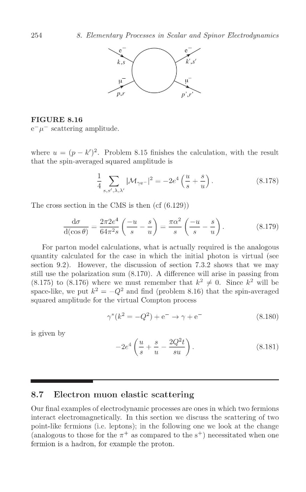
FIGURE 8.16
e
− μ
− scattering amplitude.
where u = (p − k
′ )
2 . Problem 8.15 finishes the calculation, with the result
that the spin-averaged squared amplitude is
∑
(
)
1
u
s
4
|M γe − |
2 = −2e
+
.
(8.178)
4
s
u
'
s,s ,λ,λ '
The cross section in the CMS is then (cf (6.129))
(
)
(
)
dσ
2π2e
4
−u
s
πα
2
−u
s
=
−
=
−
.
(8.179)
d(cos θ)
64π 2 s
s
u
s
s
u
For parton model calculations, what is actually required is the analogous
quantity calculated for the case in which the initial photon is virtual (see
section 9.2). However, the discussion of section 7.3.2 shows that we may
still use the polarization sum (8.170). A difference will arise in passing from
(8.175) to (8.176) where we must remember that k
2
/
will be
= 0. Since k
2
space-like, we put k
2 = −Q
2 and find (problem 8.16) that the spin-averaged
squared amplitude for the virtual Compton process
−
γ
∗ (k
2 = −Q
2 ) + e
−
→ γ + e
(8.180)
is given by
(
)
u
s
2Q
2 t
4
−2e
+ −
.
(8.181)
s
u
su
8.7 Electron muon elastic scattering
Our final examples of electrodynamic processes are ones in which two fermions
interact electromagnetically. In this section we discuss the scattering of two
point-like fermions (i.e. leptons); in the following one we look at the change
(analogous to those for the π
+ as compared to the s
+ ) necessitated when one
fermion is a hadron, for example the proton.
8. Elementary Processes in Scalar and Spinor Electrodynamics
FIGURE 8.16
e
− μ
− scattering amplitude.
where u = (p − k
′ )
2 . Problem 8.15 finishes the calculation, with the result
that the spin-averaged squared amplitude is
∑
(
)
1
u
s
4
|M γe − |
2 = −2e
+
.
(8.178)
4
s
u
'
s,s ,λ,λ '
The cross section in the CMS is then (cf (6.129))
(
)
(
)
dσ
2π2e
4
−u
s
πα
2
−u
s
=
−
=
−
.
(8.179)
d(cos θ)
64π 2 s
s
u
s
s
u
For parton model calculations, what is actually required is the analogous
quantity calculated for the case in which the initial photon is virtual (see
section 9.2). However, the discussion of section 7.3.2 shows that we may
still use the polarization sum (8.170). A difference will arise in passing from
(8.175) to (8.176) where we must remember that k
2
/
will be
= 0. Since k
2
space-like, we put k
2 = −Q
2 and find (problem 8.16) that the spin-averaged
squared amplitude for the virtual Compton process
−
γ
∗ (k
2 = −Q
2 ) + e
−
→ γ + e
(8.180)
is given by
(
)
u
s
2Q
2 t
4
−2e
+ −
.
(8.181)
s
u
su
8.7 Electron muon elastic scattering
Our final examples of electrodynamic processes are ones in which two fermions
interact electromagnetically. In this section we discuss the scattering of two
point-like fermions (i.e. leptons); in the following one we look at the change
(analogous to those for the π
+ as compared to the s
+ ) necessitated when one
fermion is a hadron, for example the proton.