

189
7.1. The complex scalar field
x
x
t
t
x 1
x 2
t 2
t 1
t 1
t 2
x 2
x 1
φ
¯
φ
(a)
(b)
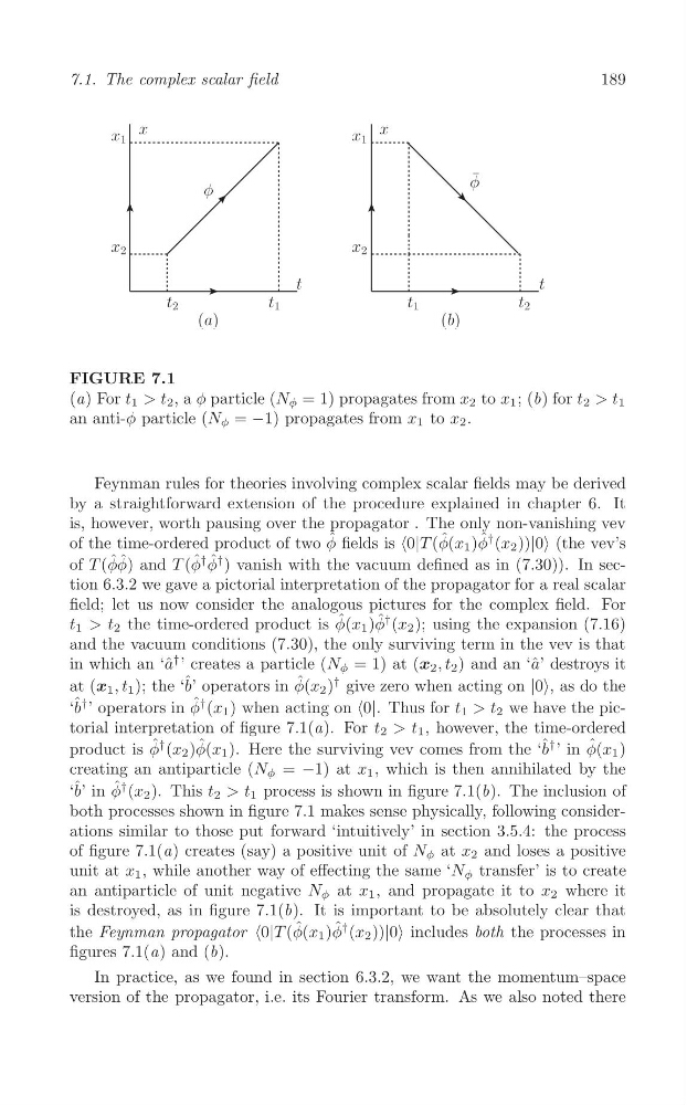
FIGURE 7.1
(a) For t 1 > t 2 , a φ particle (N φ = 1) propagates from x 2 to x 1 ; (b) for t 2 > t 1
an anti-φ particle (N φ = −1) propagates from x 1 to x 2 .
Feynman rules for theories involving complex scalar fields may be derived
by a straightforward extension of the procedure explained in chapter 6. It
is, however, worth pausing over the propagator . The only non-vanishing vev
of the time-ordered product of two φ ˆ fields is <0|T (φ ˆ (x 1 )φ ˆ† (x 2 ))|0> (the vev’s
† ˆ
of T (φ ˆ φ ˆ ) and T (φ ˆ φ
† ) vanish with the vacuum defined as in (7.30)). In section 6.3.2 we gave a pictorial interpretation of the propagator for a real scalar
field; let us now consider the analogous pictures for the complex field. For
t 1 > t 2 the time-ordered product is φ ˆ (x 1 )φ ˆ † (x 2 ); using the expansion (7.16)
and the vacuum conditions (7.30), the only surviving term in the vev is that
in which an ‘ˆ a
† ’ creates a particle (N φ = 1) at (x 2 , t 2 ) and an ‘ˆ a’ destroys it
at (x 1 , t 1 ); the ‘ ˆ b’ operators in φ ˆ (x 2 )
† give zero when acting on |0>, as do the
‘ ˆ b
† ’ operators in φ ˆ† (x 1 ) when acting on <0|. Thus for t 1 > t 2 we have the pictorial interpretation of figure 7.1(a). For t 2 > t 1 , however, the time-ordered
product is φ ˆ† (x 2 )φ ˆ (x 1 ). Here the surviving vev comes from the ‘ ˆ b
† ’ in φ ˆ (x 1 )
creating an antiparticle (N φ = −1) at x 1 , which is then annihilated by the
‘ ˆ b’ in φ ˆ † (x 2 ). This t 2 > t 1 process is shown in figure 7.1(b). The inclusion of
both processes shown in figure 7.1 makes sense physically, following considerations similar to those put forward ‘intuitively’ in section 3.5.4: the process
of figure 7.1(a) creates (say) a positive unit of N φ at x 2 and loses a positive
unit at x 1 , while another way of effecting the same ‘N φ transfer’ is to create
an antiparticle of unit negative N φ at x 1 , and propagate it to x 2 where it
is destroyed, as in figure 7.1(b). It is important to be absolutely clear that
the Feynman propagator <0|T (φ ˆ (x 1 )φ ˆ† (x 2 ))|0> includes both the processes in
figures 7.1(a) and (b).
In practice, as we found in section 6.3.2, we want the momentum–space
version of the propagator, i.e. its Fourier transform. As we also noted there
7.1. The complex scalar field
x
x
t
t
x 1
x 2
t 2
t 1
t 1
t 2
x 2
x 1
φ
¯
φ
(a)
(b)
FIGURE 7.1
(a) For t 1 > t 2 , a φ particle (N φ = 1) propagates from x 2 to x 1 ; (b) for t 2 > t 1
an anti-φ particle (N φ = −1) propagates from x 1 to x 2 .
Feynman rules for theories involving complex scalar fields may be derived
by a straightforward extension of the procedure explained in chapter 6. It
is, however, worth pausing over the propagator . The only non-vanishing vev
of the time-ordered product of two φ ˆ fields is <0|T (φ ˆ (x 1 )φ ˆ† (x 2 ))|0> (the vev’s
† ˆ
of T (φ ˆ φ ˆ ) and T (φ ˆ φ
† ) vanish with the vacuum defined as in (7.30)). In section 6.3.2 we gave a pictorial interpretation of the propagator for a real scalar
field; let us now consider the analogous pictures for the complex field. For
t 1 > t 2 the time-ordered product is φ ˆ (x 1 )φ ˆ † (x 2 ); using the expansion (7.16)
and the vacuum conditions (7.30), the only surviving term in the vev is that
in which an ‘ˆ a
† ’ creates a particle (N φ = 1) at (x 2 , t 2 ) and an ‘ˆ a’ destroys it
at (x 1 , t 1 ); the ‘ ˆ b’ operators in φ ˆ (x 2 )
† give zero when acting on |0>, as do the
‘ ˆ b
† ’ operators in φ ˆ† (x 1 ) when acting on <0|. Thus for t 1 > t 2 we have the pictorial interpretation of figure 7.1(a). For t 2 > t 1 , however, the time-ordered
product is φ ˆ† (x 2 )φ ˆ (x 1 ). Here the surviving vev comes from the ‘ ˆ b
† ’ in φ ˆ (x 1 )
creating an antiparticle (N φ = −1) at x 1 , which is then annihilated by the
‘ ˆ b’ in φ ˆ † (x 2 ). This t 2 > t 1 process is shown in figure 7.1(b). The inclusion of
both processes shown in figure 7.1 makes sense physically, following considerations similar to those put forward ‘intuitively’ in section 3.5.4: the process
of figure 7.1(a) creates (say) a positive unit of N φ at x 2 and loses a positive
unit at x 1 , while another way of effecting the same ‘N φ transfer’ is to create
an antiparticle of unit negative N φ at x 1 , and propagate it to x 2 where it
is destroyed, as in figure 7.1(b). It is important to be absolutely clear that
the Feynman propagator <0|T (φ ˆ (x 1 )φ ˆ† (x 2 ))|0> includes both the processes in
figures 7.1(a) and (b).
In practice, as we found in section 6.3.2, we want the momentum–space
version of the propagator, i.e. its Fourier transform. As we also noted there