

190
7. Quantum Field Theory III
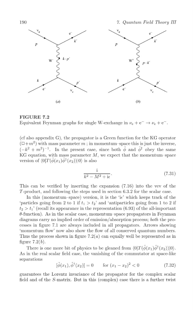
FIGURE 7.2
Equivalent Feynman graphs for single W-exchange in ν e + e
−
→ ν e + e
− .
(cf also appendix G), the propagator is a Green function for the KG operator
(❗+m
2 ) with mass parameter m ; in momentum–space this is just the inverse,
2
2 )
−1
†
(−k + m
. In the present case, since both φ ˆ and φ ˆ obey the same
KG equation, with mass parameter M , we expect that the momentum–space
version of <0|T (φ ˆ (x 1 )φ ˆ † (x 2 ))|0> is also
i
.
(7.31)
k 2 − M 2 + i∈
This can be verified by inserting the expansion (7.16) into the vev of the
T -product, and following the steps used in section 6.3.2 for the scalar case.
In this (momentum–space) version, it is the ‘i∈’ which keeps track of the
‘particles going from 2 to 1 if t 1 > t 2 ’ and ‘antiparticles going from 1 to 2 if
t 2 > t 1 ’ (recall its appearance in the representation (6.93) of the all-important
θ-function). As in the scalar case, momentum–space propagators in Feynman
diagrams carry no implied order of emission/absorption process; both the processes in figure 7.1 are always included in all propagators. Arrows showing
‘momentum flow’ now also show the flow of all conserved quantum numbers.
Thus the process shown in figure 7.2(a) can equally well be represented as in
figure 7.2(b).
There is one more bit of physics to be gleaned from <0|T (φ ˆ (x 1 )φ ˆ† (x 2 ))|0>.
As in the real scalar field case, the vanishing of the commutator at space-like
separations
[φ ˆ (x 1 ), φ ˆ † (x 2 )] = 0
for (x 1 − x 2 )
2 < 0
(7.32)
guarantees the Lorentz invariance of the propagator for the complex scalar
field and of the S-matrix. But in this (complex) case there is a further twist
7. Quantum Field Theory III
FIGURE 7.2
Equivalent Feynman graphs for single W-exchange in ν e + e
−
→ ν e + e
− .
(cf also appendix G), the propagator is a Green function for the KG operator
(❗+m
2 ) with mass parameter m ; in momentum–space this is just the inverse,
2
2 )
−1
†
(−k + m
. In the present case, since both φ ˆ and φ ˆ obey the same
KG equation, with mass parameter M , we expect that the momentum–space
version of <0|T (φ ˆ (x 1 )φ ˆ † (x 2 ))|0> is also
i
.
(7.31)
k 2 − M 2 + i∈
This can be verified by inserting the expansion (7.16) into the vev of the
T -product, and following the steps used in section 6.3.2 for the scalar case.
In this (momentum–space) version, it is the ‘i∈’ which keeps track of the
‘particles going from 2 to 1 if t 1 > t 2 ’ and ‘antiparticles going from 1 to 2 if
t 2 > t 1 ’ (recall its appearance in the representation (6.93) of the all-important
θ-function). As in the scalar case, momentum–space propagators in Feynman
diagrams carry no implied order of emission/absorption process; both the processes in figure 7.1 are always included in all propagators. Arrows showing
‘momentum flow’ now also show the flow of all conserved quantum numbers.
Thus the process shown in figure 7.2(a) can equally well be represented as in
figure 7.2(b).
There is one more bit of physics to be gleaned from <0|T (φ ˆ (x 1 )φ ˆ† (x 2 ))|0>.
As in the real scalar field case, the vanishing of the commutator at space-like
separations
[φ ˆ (x 1 ), φ ˆ † (x 2 )] = 0
for (x 1 − x 2 )
2 < 0
(7.32)
guarantees the Lorentz invariance of the propagator for the complex scalar
field and of the S-matrix. But in this (complex) case there is a further twist