

178
6. Quantum Field Theory II: Interacting Scalar Fields
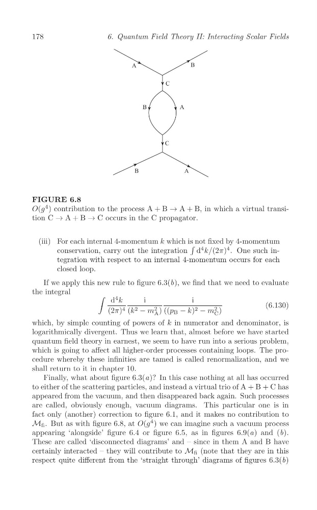
FIGURE 6.8
O(g
4 ) contribution to the process A + B → A + B, in which a virtual transition C → A + B → C occurs in the C propagator.
(iii) For each internal 4-momentum k which is not fixed by 4-momentum
∫
conservation, carry out the integration d
4 k/(2π)
4 . One such integration with respect to an internal 4-momentum occurs for each
closed loop.
If we apply this new rule to figure 6.3(b), we find that we need to evaluate
the integral
∫ d
4 k
i
i
(6.130)
2
2
(2π) 4 (k 2 − m ) ((p B − k) 2 − m )
A
C
which, by simple counting of powers of k in numerator and denominator, is
logarithmically divergent. Thus we learn that, almost before we have started
quantum field theory in earnest, we seem to have run into a serious problem,
which is going to affect all higher-order processes containing loops. The procedure whereby these infinities are tamed is called renormalization, and we
shall return to it in chapter 10.
Finally, what about figure 6.3(a)? In this case nothing at all has occurred
to either of the scattering particles, and instead a virtual trio of A + B + C has
appeared from the vacuum, and then disappeared back again. Such processes
are called, obviously enough, vacuum diagrams. This particular one is in
fact only (another) correction to figure 6.1, and it makes no contribution to
M fi . But as with figure 6.8, at O(g
4 ) we can imagine such a vacuum process
appearing ‘alongside’ figure 6.4 or figure 6.5, as in figures 6.9(a) and (b).
These are called ‘disconnected diagrams’ and – since in them A and B have
certainly interacted – they will contribute to M fi (note that they are in this
respect quite different from the ‘straight through’ diagrams of figures 6.3(b)
6. Quantum Field Theory II: Interacting Scalar Fields
FIGURE 6.8
O(g
4 ) contribution to the process A + B → A + B, in which a virtual transition C → A + B → C occurs in the C propagator.
(iii) For each internal 4-momentum k which is not fixed by 4-momentum
∫
conservation, carry out the integration d
4 k/(2π)
4 . One such integration with respect to an internal 4-momentum occurs for each
closed loop.
If we apply this new rule to figure 6.3(b), we find that we need to evaluate
the integral
∫ d
4 k
i
i
(6.130)
2
2
(2π) 4 (k 2 − m ) ((p B − k) 2 − m )
A
C
which, by simple counting of powers of k in numerator and denominator, is
logarithmically divergent. Thus we learn that, almost before we have started
quantum field theory in earnest, we seem to have run into a serious problem,
which is going to affect all higher-order processes containing loops. The procedure whereby these infinities are tamed is called renormalization, and we
shall return to it in chapter 10.
Finally, what about figure 6.3(a)? In this case nothing at all has occurred
to either of the scattering particles, and instead a virtual trio of A + B + C has
appeared from the vacuum, and then disappeared back again. Such processes
are called, obviously enough, vacuum diagrams. This particular one is in
fact only (another) correction to figure 6.1, and it makes no contribution to
M fi . But as with figure 6.8, at O(g
4 ) we can imagine such a vacuum process
appearing ‘alongside’ figure 6.4 or figure 6.5, as in figures 6.9(a) and (b).
These are called ‘disconnected diagrams’ and – since in them A and B have
certainly interacted – they will contribute to M fi (note that they are in this
respect quite different from the ‘straight through’ diagrams of figures 6.3(b)