

|
177
6.3. Applications to the ‘ABC’ theory
and a straightforward calculation shows that
2
2
(p A · p B )
2
− m
= p
2 W
2 .
A m B
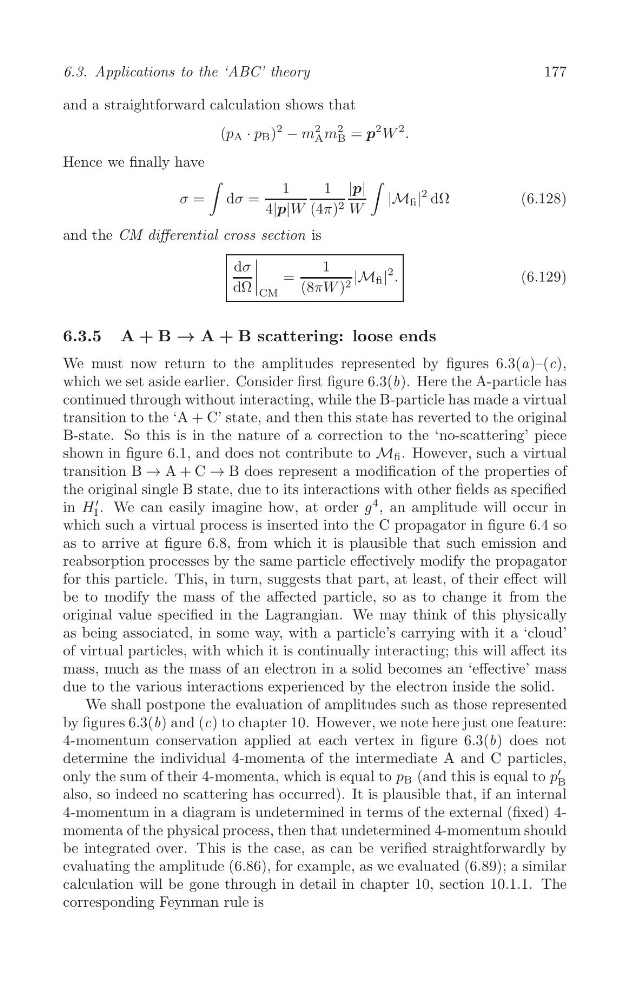
Hence we finally have
∫
∫
σ = dσ =
1
4|p|W
1
(4π) 2
|p|
W
|M fi |
2 dΩ
(6.128)
and the CM differential cross section is
dσ
1
=
|M fi |
2 .
(6.129)
dΩ
|
|
|
(8πW ) 2
CM
6.3.5 A + B → A + B scattering: loose ends
We must now return to the amplitudes represented by figures 6.3(a)–(c),
which we set aside earlier. Consider first figure 6.3(b). Here the A-particle has
continued through without interacting, while the B-particle has made a virtual
transition to the ‘A + C’ state, and then this state has reverted to the original
B-state. So this is in the nature of a correction to the ‘no-scattering’ piece
shown in figure 6.1, and does not contribute to M fi . However, such a virtual
transition B → A + C → B does represent a modification of the properties of
the original single B state, due to its interactions with other fields as specified
in H I
′ . We can easily imagine how, at order g
4 , an amplitude will occur in
which such a virtual process is inserted into the C propagator in figure 6.4 so
as to arrive at figure 6.8, from which it is plausible that such emission and
reabsorption processes by the same particle effectively modify the propagator
for this particle. This, in turn, suggests that part, at least, of their effect will
be to modify the mass of the affected particle, so as to change it from the
original value specified in the Lagrangian. We may think of this physically
as being associated, in some way, with a particle’s carrying with it a ‘cloud’
of virtual particles, with which it is continually interacting; this will affect its
mass, much as the mass of an electron in a solid becomes an ‘effective’ mass
due to the various interactions experienced by the electron inside the solid.
We shall postpone the evaluation of amplitudes such as those represented
by figures 6.3(b) and (c) to chapter 10. However, we note here just one feature:
4-momentum conservation applied at each vertex in figure 6.3(b) does not
determine the individual 4-momenta of the intermediate A and C particles,
′
only the sum of their 4-momenta, which is equal to p B (and this is equal to p B
also, so indeed no scattering has occurred). It is plausible that, if an internal
4-momentum in a diagram is undetermined in terms of the external (fixed) 4momenta of the physical process, then that undetermined 4-momentum should
be integrated over. This is the case, as can be verified straightforwardly by
evaluating the amplitude (6.86), for example, as we evaluated (6.89); a similar
calculation will be gone through in detail in chapter 10, section 10.1.1. The
corresponding Feynman rule is
177
6.3. Applications to the ‘ABC’ theory
and a straightforward calculation shows that
2
2
(p A · p B )
2
− m
= p
2 W
2 .
A m B
Hence we finally have
∫
∫
σ = dσ =
1
4|p|W
1
(4π) 2
|p|
W
|M fi |
2 dΩ
(6.128)
and the CM differential cross section is
dσ
1
=
|M fi |
2 .
(6.129)
dΩ
|
|
|
(8πW ) 2
CM
6.3.5 A + B → A + B scattering: loose ends
We must now return to the amplitudes represented by figures 6.3(a)–(c),
which we set aside earlier. Consider first figure 6.3(b). Here the A-particle has
continued through without interacting, while the B-particle has made a virtual
transition to the ‘A + C’ state, and then this state has reverted to the original
B-state. So this is in the nature of a correction to the ‘no-scattering’ piece
shown in figure 6.1, and does not contribute to M fi . However, such a virtual
transition B → A + C → B does represent a modification of the properties of
the original single B state, due to its interactions with other fields as specified
in H I
′ . We can easily imagine how, at order g
4 , an amplitude will occur in
which such a virtual process is inserted into the C propagator in figure 6.4 so
as to arrive at figure 6.8, from which it is plausible that such emission and
reabsorption processes by the same particle effectively modify the propagator
for this particle. This, in turn, suggests that part, at least, of their effect will
be to modify the mass of the affected particle, so as to change it from the
original value specified in the Lagrangian. We may think of this physically
as being associated, in some way, with a particle’s carrying with it a ‘cloud’
of virtual particles, with which it is continually interacting; this will affect its
mass, much as the mass of an electron in a solid becomes an ‘effective’ mass
due to the various interactions experienced by the electron inside the solid.
We shall postpone the evaluation of amplitudes such as those represented
by figures 6.3(b) and (c) to chapter 10. However, we note here just one feature:
4-momentum conservation applied at each vertex in figure 6.3(b) does not
determine the individual 4-momenta of the intermediate A and C particles,
′
only the sum of their 4-momenta, which is equal to p B (and this is equal to p B
also, so indeed no scattering has occurred). It is plausible that, if an internal
4-momentum in a diagram is undetermined in terms of the external (fixed) 4momenta of the physical process, then that undetermined 4-momentum should
be integrated over. This is the case, as can be verified straightforwardly by
evaluating the amplitude (6.86), for example, as we evaluated (6.89); a similar
calculation will be gone through in detail in chapter 10, section 10.1.1. The
corresponding Feynman rule is