

174
6. Quantum Field Theory II: Interacting Scalar Fields
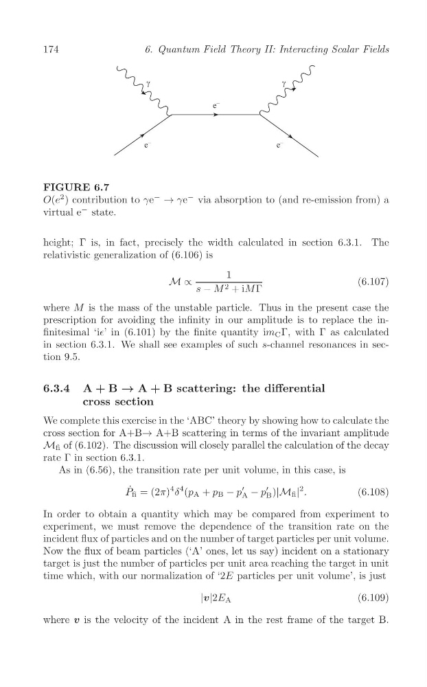
FIGURE 6.7
O(e
2 ) contribution to γe
−
→ γe
− via absorption to (and re-emission from) a
virtual e
− state.
height; Γ is, in fact, precisely the width calculated in section 6.3.1. The
relativistic generalization of (6.106) is
1
M ∝
(6.107)
s − M 2 + iM Γ
where M is the mass of the unstable particle. Thus in the present case the
prescription for avoiding the infinity in our amplitude is to replace the infinitesimal ‘i∈’ in (6.101) by the finite quantity im C Γ, with Γ as calculated
in section 6.3.1. We shall see examples of such s-channel resonances in section 9.5.
6.3.4 A + B → A + B scattering: the differential
cross section
We complete this exercise in the ‘ABC’ theory by showing how to calculate the
cross section for A+B→ A+B scattering in terms of the invariant amplitude
M fi of (6.102). The discussion will closely parallel the calculation of the decay
rate Γ in section 6.3.1.
As in (6.56), the transition rate per unit volume, in this case, is
˙
′
′
P fi = (2π)
4 δ
4 (p A + p B − p A − p B )|M fi |
2 .
(6.108)
In order to obtain a quantity which may be compared from experiment to
experiment, we must remove the dependence of the transition rate on the
incident flux of particles and on the number of target particles per unit volume.
Now the flux of beam particles (‘A’ ones, let us say) incident on a stationary
target is just the number of particles per unit area reaching the target in unit
time which, with our normalization of ‘2E particles per unit volume’, is just
|v|2E A
(6.109)
where v is the velocity of the incident A in the rest frame of the target B.
6. Quantum Field Theory II: Interacting Scalar Fields
FIGURE 6.7
O(e
2 ) contribution to γe
−
→ γe
− via absorption to (and re-emission from) a
virtual e
− state.
height; Γ is, in fact, precisely the width calculated in section 6.3.1. The
relativistic generalization of (6.106) is
1
M ∝
(6.107)
s − M 2 + iM Γ
where M is the mass of the unstable particle. Thus in the present case the
prescription for avoiding the infinity in our amplitude is to replace the infinitesimal ‘i∈’ in (6.101) by the finite quantity im C Γ, with Γ as calculated
in section 6.3.1. We shall see examples of such s-channel resonances in section 9.5.
6.3.4 A + B → A + B scattering: the differential
cross section
We complete this exercise in the ‘ABC’ theory by showing how to calculate the
cross section for A+B→ A+B scattering in terms of the invariant amplitude
M fi of (6.102). The discussion will closely parallel the calculation of the decay
rate Γ in section 6.3.1.
As in (6.56), the transition rate per unit volume, in this case, is
˙
′
′
P fi = (2π)
4 δ
4 (p A + p B − p A − p B )|M fi |
2 .
(6.108)
In order to obtain a quantity which may be compared from experiment to
experiment, we must remove the dependence of the transition rate on the
incident flux of particles and on the number of target particles per unit volume.
Now the flux of beam particles (‘A’ ones, let us say) incident on a stationary
target is just the number of particles per unit area reaching the target in unit
time which, with our normalization of ‘2E particles per unit volume’, is just
|v|2E A
(6.109)
where v is the velocity of the incident A in the rest frame of the target B.