

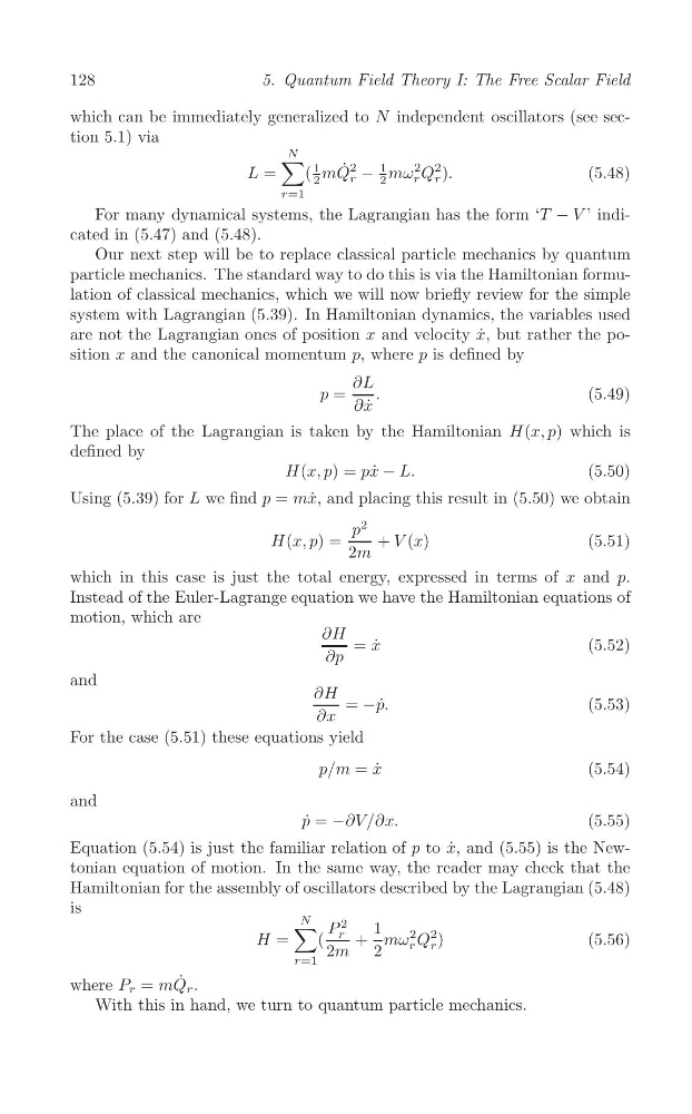
128
5. Quantum Field Theory I: The Free Scalar Field
which can be immediately generalized to N independent oscillators (see section 5.1) via
N
∑
L =
(
1 mQ ˙ 2 −
1 mω
2 Q
2 ).
(5.48)
2
r
2
r r
r=1
For many dynamical systems, the Lagrangian has the form ‘T − V ’ indicated in (5.47) and (5.48).
Our next step will be to replace classical particle mechanics by quantum
particle mechanics. The standard way to do this is via the Hamiltonian formulation of classical mechanics, which we will now briefly review for the simple
system with Lagrangian (5.39). In Hamiltonian dynamics, the variables used
are not the Lagrangian ones of position x and velocity ˙
x, but rather the position x and the canonical momentum p, where p is defined by
∂L
p =
.
(5.49)
∂x ˙
The place of the Lagrangian is taken by the Hamiltonian H(x, p) which is
defined by
H(x, p) = px ˙ − L.
(5.50)
Using (5.39) for L we find p = mx ˙ , and placing this result in (5.50) we obtain
2
p
H(x, p) =
+ V (x)
(5.51)
2m
which in this case is just the total energy, expressed in terms of x and p.
Instead of the Euler-Lagrange equation we have the Hamiltonian equations of
motion, which are
∂H = ˙
x
(5.52)
∂p
and
∂H = −p. ˙
(5.53)
∂x
For the case (5.51) these equations yield
p/m = ˙
x
(5.54)
and
p ˙ = −∂V/∂x.
(5.55)
Equation (5.54) is just the familiar relation of p to ˙
x, and (5.55) is the Newtonian equation of motion. In the same way, the reader may check that the
Hamiltonian for the assembly of oscillators described by the Lagrangian (5.48)
is
N
∑ P
2
r
H =
(
+
1 mω
2 Q
2 )
(5.56)
r r
2m 2
r=1
˙
where P r = mQ r .
With this in hand, we turn to quantum particle mechanics.
5. Quantum Field Theory I: The Free Scalar Field
which can be immediately generalized to N independent oscillators (see section 5.1) via
N
∑
L =
(
1 mQ ˙ 2 −
1 mω
2 Q
2 ).
(5.48)
2
r
2
r r
r=1
For many dynamical systems, the Lagrangian has the form ‘T − V ’ indicated in (5.47) and (5.48).
Our next step will be to replace classical particle mechanics by quantum
particle mechanics. The standard way to do this is via the Hamiltonian formulation of classical mechanics, which we will now briefly review for the simple
system with Lagrangian (5.39). In Hamiltonian dynamics, the variables used
are not the Lagrangian ones of position x and velocity ˙
x, but rather the position x and the canonical momentum p, where p is defined by
∂L
p =
.
(5.49)
∂x ˙
The place of the Lagrangian is taken by the Hamiltonian H(x, p) which is
defined by
H(x, p) = px ˙ − L.
(5.50)
Using (5.39) for L we find p = mx ˙ , and placing this result in (5.50) we obtain
2
p
H(x, p) =
+ V (x)
(5.51)
2m
which in this case is just the total energy, expressed in terms of x and p.
Instead of the Euler-Lagrange equation we have the Hamiltonian equations of
motion, which are
∂H = ˙
x
(5.52)
∂p
and
∂H = −p. ˙
(5.53)
∂x
For the case (5.51) these equations yield
p/m = ˙
x
(5.54)
and
p ˙ = −∂V/∂x.
(5.55)
Equation (5.54) is just the familiar relation of p to ˙
x, and (5.55) is the Newtonian equation of motion. In the same way, the reader may check that the
Hamiltonian for the assembly of oscillators described by the Lagrangian (5.48)
is
N
∑ P
2
r
H =
(
+
1 mω
2 Q
2 )
(5.56)
r r
2m 2
r=1
˙
where P r = mQ r .
With this in hand, we turn to quantum particle mechanics.