

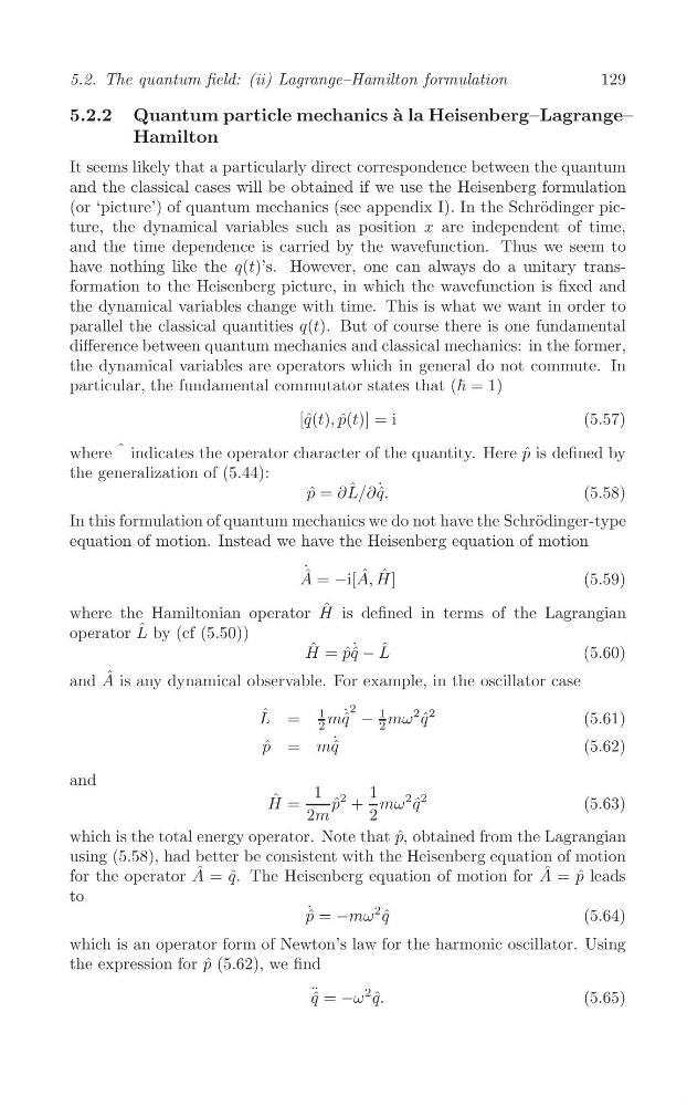
129
5.2. The quantum field: (ii) Lagrange–Hamilton formulation
5.2.2 Quantum particle mechanics ` a la Heisenberg–Lagrange–
Hamilton
It seems likely that a particularly direct correspondence between the quantum
and the classical cases will be obtained if we use the Heisenberg formulation
(or ‘picture’) of quantum mechanics (see appendix I). In the Schr¨ odinger picture, the dynamical variables such as position x are independent of time,
and the time dependence is carried by the wavefunction. Thus we seem to
have nothing like the q(t)’s. However, one can always do a unitary transformation to the Heisenberg picture, in which the wavefunction is fixed and
the dynamical variables change with time. This is what we want in order to
parallel the classical quantities q(t). But of course there is one fundamental
difference between quantum mechanics and classical mechanics: in the former,
the dynamical variables are operators which in general do not commute. In
particular, the fundamental commutator states that (ħ = 1)
[ˆ q(t), p ˆ(t)] = i
(5.57)
where ˆ indicates the operator character of the quantity. Here ˆ
p is defined by
the generalization of (5.44):
∂ ˆ
p ˆ = L/∂q. ˆ ˙
(5.58)
In this formulation of quantum mechanics we do not have the Schr¨ odinger-type
equation of motion. Instead we have the Heisenberg equation of motion
˙ ˆ
A =
A, ˆ
(5.59)
−i[ ˆ H]
where the Hamiltonian operator H ˆ is defined in terms of the Lagrangian
operator L ˆ by (cf (5.50))
H ˆ = ˆ
pq ˆ ˙ − L ˆ
(5.60)
and A ˆ is any dynamical observable. For example, in the oscillator case
2
ˆ
1
˙ −
1
2
L = mq ˆ
mω
2 q ˆ
(5.61)
2
2
˙
p ˆ = mq ˆ
(5.62)
and
ˆ
2
2
1
1 mω
2 q ˆ
(5.63)
H = p ˆ +
2m
2
which is the total energy operator. Note that ˆ
p, obtained from the Lagrangian
using (5.58), had better be consistent with the Heisenberg equation of motion
for the operator A ˆ = ˆ
q. The Heisenberg equation of motion for A ˆ = ˆ
p leads
to
p ˆ ˙ = −mω
2 q ˆ
(5.64)
which is an operator form of Newton’s law for the harmonic oscillator. Using
the expression for ˆ
p (5.62), we find
¨ q ˆ = −ω
2 q. ˆ
(5.65)
5.2. The quantum field: (ii) Lagrange–Hamilton formulation
5.2.2 Quantum particle mechanics ` a la Heisenberg–Lagrange–
Hamilton
It seems likely that a particularly direct correspondence between the quantum
and the classical cases will be obtained if we use the Heisenberg formulation
(or ‘picture’) of quantum mechanics (see appendix I). In the Schr¨ odinger picture, the dynamical variables such as position x are independent of time,
and the time dependence is carried by the wavefunction. Thus we seem to
have nothing like the q(t)’s. However, one can always do a unitary transformation to the Heisenberg picture, in which the wavefunction is fixed and
the dynamical variables change with time. This is what we want in order to
parallel the classical quantities q(t). But of course there is one fundamental
difference between quantum mechanics and classical mechanics: in the former,
the dynamical variables are operators which in general do not commute. In
particular, the fundamental commutator states that (ħ = 1)
[ˆ q(t), p ˆ(t)] = i
(5.57)
where ˆ indicates the operator character of the quantity. Here ˆ
p is defined by
the generalization of (5.44):
∂ ˆ
p ˆ = L/∂q. ˆ ˙
(5.58)
In this formulation of quantum mechanics we do not have the Schr¨ odinger-type
equation of motion. Instead we have the Heisenberg equation of motion
˙ ˆ
A =
A, ˆ
(5.59)
−i[ ˆ H]
where the Hamiltonian operator H ˆ is defined in terms of the Lagrangian
operator L ˆ by (cf (5.50))
H ˆ = ˆ
pq ˆ ˙ − L ˆ
(5.60)
and A ˆ is any dynamical observable. For example, in the oscillator case
2
ˆ
1
˙ −
1
2
L = mq ˆ
mω
2 q ˆ
(5.61)
2
2
˙
p ˆ = mq ˆ
(5.62)
and
ˆ
2
2
1
1 mω
2 q ˆ
(5.63)
H = p ˆ +
2m
2
which is the total energy operator. Note that ˆ
p, obtained from the Lagrangian
using (5.58), had better be consistent with the Heisenberg equation of motion
for the operator A ˆ = ˆ
q. The Heisenberg equation of motion for A ˆ = ˆ
p leads
to
p ˆ ˙ = −mω
2 q ˆ
(5.64)
which is an operator form of Newton’s law for the harmonic oscillator. Using
the expression for ˆ
p (5.62), we find
¨ q ˆ = −ω
2 q. ˆ
(5.65)