

127
5.2. The quantum field: (ii) Lagrange–Hamilton formulation
Our problem is something like the familiar one of finding the point t 0 at
which a certain function f (t) has a stationary value. In the present case,
however, the function S is not a simple function of t – rather it is a function
of the entire set of points q(t). It is a function of the function q(t), or a
‘f unctional’ of q(t). We want to know what particular ‘q c (t)’ minimizes S.
By analogy with the single-variable case, we consider a small variation δq(t)
in the path from q(t 1 ) to q(t 2 ). At the minimum, the change δS corresponding
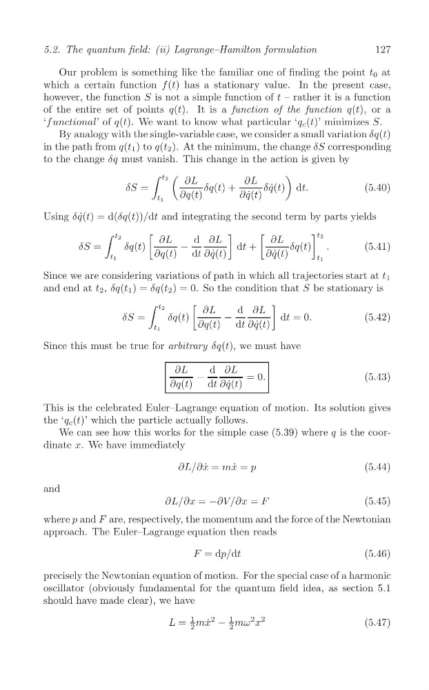
to the change δq must vanish. This change in the action is given by
(
)
∫ t2
∂L
∂L
δS =
δq(t) +
δq˙(t) dt.
(5.40)
t1
∂q(t)
∂q˙(t)
Using δq˙(t) = d(δq(t))/dt and integrating the second term by parts yields
∫
[
]
[
] t2
t2
∂L
d ∂L
∂L
δS =
δq(t)
−
dt +
δq(t) .
(5.41)
t1
∂q(t) dt ∂q˙(t)
∂q˙(t)
t1
Since we are considering variations of path in which all trajectories start at t 1
and end at t 2 , δq(t 1 ) = δq(t 2 ) = 0. So the condition that S be stationary is
∫
[
]
t2
∂L
d ∂L
δS =
δq(t)
−
dt = 0.
(5.42)
∂q(t) dt ∂q˙(t)
t1
Since this must be true for arbitrary δq(t), we must have
∂L
d ∂L
−
= 0.
(5.43)
∂q(t) dt ∂q˙(t)
This is the celebrated Euler–Lagrange equation of motion. Its solution gives
the ‘q c (t)’ which the particle actually follows.
We can see how this works for the simple case (5.39) where q is the coordinate x. We have immediately
∂L/∂x ˙ = mx ˙ = p
(5.44)
and
∂L/∂x = −∂V/∂x = F
(5.45)
where p and F are, respectively, the momentum and the force of the Newtonian
approach. The Euler–Lagrange equation then reads
F = dp/dt
(5.46)
precisely the Newtonian equation of motion. For the special case of a harmonic
oscillator (obviously fundamental for the quantum field idea, as section 5.1
should have made clear), we have
1
2
−
1
2
L = mx ˙
mω
2 x
(5.47)
2
2
5.2. The quantum field: (ii) Lagrange–Hamilton formulation
Our problem is something like the familiar one of finding the point t 0 at
which a certain function f (t) has a stationary value. In the present case,
however, the function S is not a simple function of t – rather it is a function
of the entire set of points q(t). It is a function of the function q(t), or a
‘f unctional’ of q(t). We want to know what particular ‘q c (t)’ minimizes S.
By analogy with the single-variable case, we consider a small variation δq(t)
in the path from q(t 1 ) to q(t 2 ). At the minimum, the change δS corresponding
to the change δq must vanish. This change in the action is given by
(
)
∫ t2
∂L
∂L
δS =
δq(t) +
δq˙(t) dt.
(5.40)
t1
∂q(t)
∂q˙(t)
Using δq˙(t) = d(δq(t))/dt and integrating the second term by parts yields
∫
[
]
[
] t2
t2
∂L
d ∂L
∂L
δS =
δq(t)
−
dt +
δq(t) .
(5.41)
t1
∂q(t) dt ∂q˙(t)
∂q˙(t)
t1
Since we are considering variations of path in which all trajectories start at t 1
and end at t 2 , δq(t 1 ) = δq(t 2 ) = 0. So the condition that S be stationary is
∫
[
]
t2
∂L
d ∂L
δS =
δq(t)
−
dt = 0.
(5.42)
∂q(t) dt ∂q˙(t)
t1
Since this must be true for arbitrary δq(t), we must have
∂L
d ∂L
−
= 0.
(5.43)
∂q(t) dt ∂q˙(t)
This is the celebrated Euler–Lagrange equation of motion. Its solution gives
the ‘q c (t)’ which the particle actually follows.
We can see how this works for the simple case (5.39) where q is the coordinate x. We have immediately
∂L/∂x ˙ = mx ˙ = p
(5.44)
and
∂L/∂x = −∂V/∂x = F
(5.45)
where p and F are, respectively, the momentum and the force of the Newtonian
approach. The Euler–Lagrange equation then reads
F = dp/dt
(5.46)
precisely the Newtonian equation of motion. For the special case of a harmonic
oscillator (obviously fundamental for the quantum field idea, as section 5.1
should have made clear), we have
1
2
−
1
2
L = mx ˙
mω
2 x
(5.47)
2
2