

126
5. Quantum Field Theory I: The Free Scalar Field
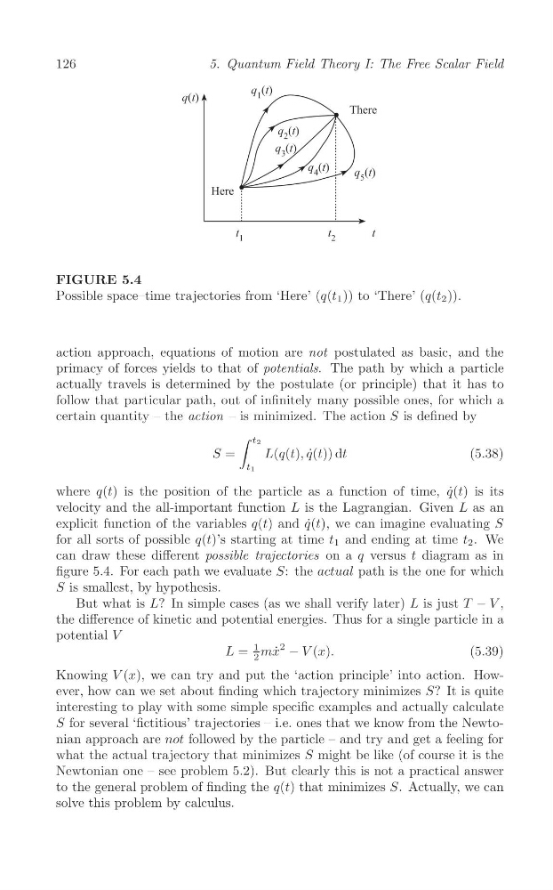
FIGURE 5.4
Possible space–time trajectories from ‘Here’ (q(t 1 )) to ‘There’ (q(t 2 )).
action approach, equations of motion are not postulated as basic, and the
primacy of forces yields to that of potentials. The path by which a particle
actually travels is determined by the postulate (or principle) that it has to
follow that particular path, out of infinitely many possible ones, for which a
certain quantity – the action – is minimized. The action S is defined by
∫ t2
S =
L(q(t), q˙(t)) dt
(5.38)
t1
where q(t) is the position of the particle as a function of time, ˙
q(t) is its
velocity and the all-important function L is the Lagrangian. Given L as an
explicit function of the variables q(t) and ˙
q(t), we can imagine evaluating S
for all sorts of possible q(t)’s starting at time t 1 and ending at time t 2 . We
can draw these different possible trajectories on a q versus t diagram as in
figure 5.4. For each path we evaluate S: the actual path is the one for which
S is smallest, by hypothesis.
But what is L? In simple cases (as we shall verify later) L is just T − V ,
the difference of kinetic and potential energies. Thus for a single particle in a
potential V
1
L = mx ˙
2
− V (x).
(5.39)
2
Knowing V (x), we can try and put the ‘action principle’ into action. However, how can we set about finding which trajectory minimizes S? It is quite
interesting to play with some simple specific examples and actually calculate
S for several ‘fictitious’ trajectories – i.e. ones that we know from the Newtonian approach are not followed by the particle – and try and get a feeling for
what the actual trajectory that minimizes S might be like (of course it is the
Newtonian one – see problem 5.2). But clearly this is not a practical answer
to the general problem of finding the q(t) that minimizes S. Actually, we can
solve this problem by calculus.
5. Quantum Field Theory I: The Free Scalar Field
FIGURE 5.4
Possible space–time trajectories from ‘Here’ (q(t 1 )) to ‘There’ (q(t 2 )).
action approach, equations of motion are not postulated as basic, and the
primacy of forces yields to that of potentials. The path by which a particle
actually travels is determined by the postulate (or principle) that it has to
follow that particular path, out of infinitely many possible ones, for which a
certain quantity – the action – is minimized. The action S is defined by
∫ t2
S =
L(q(t), q˙(t)) dt
(5.38)
t1
where q(t) is the position of the particle as a function of time, ˙
q(t) is its
velocity and the all-important function L is the Lagrangian. Given L as an
explicit function of the variables q(t) and ˙
q(t), we can imagine evaluating S
for all sorts of possible q(t)’s starting at time t 1 and ending at time t 2 . We
can draw these different possible trajectories on a q versus t diagram as in
figure 5.4. For each path we evaluate S: the actual path is the one for which
S is smallest, by hypothesis.
But what is L? In simple cases (as we shall verify later) L is just T − V ,
the difference of kinetic and potential energies. Thus for a single particle in a
potential V
1
L = mx ˙
2
− V (x).
(5.39)
2
Knowing V (x), we can try and put the ‘action principle’ into action. However, how can we set about finding which trajectory minimizes S? It is quite
interesting to play with some simple specific examples and actually calculate
S for several ‘fictitious’ trajectories – i.e. ones that we know from the Newtonian approach are not followed by the particle – and try and get a feeling for
what the actual trajectory that minimizes S might be like (of course it is the
Newtonian one – see problem 5.2). But clearly this is not a practical answer
to the general problem of finding the q(t) that minimizes S. Actually, we can
solve this problem by calculus.