

118
5. Quantum Field Theory I: The Free Scalar Field
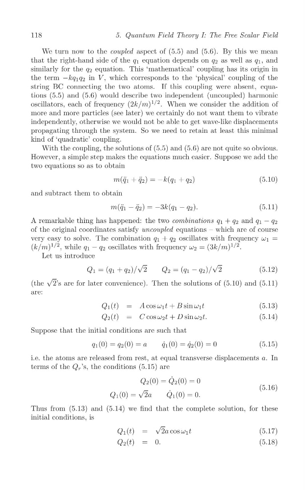
We turn now to the coupled aspect of (5.5) and (5.6). By this we mean
that the right-hand side of the q 1 equation depends on q 2 as well as q 1 , and
similarly for the q 2 equation. This ‘mathematical’ coupling has its origin in
the term −kq 1 q 2 in V , which corresponds to the ‘physical’ coupling of the
string BC connecting the two atoms. If this coupling were absent, equations (5.5) and (5.6) would describe two independent (uncoupled) harmonic
oscillators, each of frequency (2k/m)
1/2 . When we consider the addition of
more and more particles (see later) we certainly do not want them to vibrate
independently, otherwise we would not be able to get wave-like displacements
propagating through the system. So we need to retain at least this minimal
kind of ‘quadratic’ coupling.
With the coupling, the solutions of (5.5) and (5.6) are not quite so obvious.
However, a simple step makes the equations much easier. Suppose we add the
two equations so as to obtain
m(¨ q 1 + ¨
q 2 ) = −k(q 1 + q 2 )
(5.10)
and subtract them to obtain
m(¨ q 1 − q ¨ 2 ) = −3k(q 1 − q 2 ).
(5.11)
A remarkable thing has happened: the two combinations q 1 + q 2 and q 1 − q 2
of the original coordinates satisfy uncoupled equations – which are of course
very easy to solve. The combination q 1 + q 2 oscillates with frequency ω 1 =
(k/m)
1/2 , while q 1 − q 2 oscillates with frequency ω 2 = (3k/m)
1/2 .
Let us introduce
√
√
Q 1 = (q 1 + q 2 )/ 2
Q 2 = (q 1 − q 2 )/ 2
(5.12)
√
(the 2’s are for later convenience). Then the solutions of (5.10) and (5.11)
are:
Q 1 (t) = A cos ω 1 t + B sin ω 1 t
(5.13)
Q 2 (t) = C cos ω 2 t + D sin ω 2 t.
(5.14)
Suppose that the initial conditions are such that
q 1 (0) = q 2 (0) = a
q˙ 1 (0) = ˙
q 2 (0) = 0
(5.15)
i.e. the atoms are released from rest, at equal transverse displacements a. In
terms of the Q r ’s, the conditions (5.15) are
˙
Q 2 (0) = Q 2 (0) = 0
(5.16)
√
˙
Q 1 (0) = 2a
Q 1 (0) = 0.
Thus from (5.13) and (5.14) we find that the complete solution, for these
initial conditions, is
√
Q 1 (t) =
2a cos ω 1 t
(5.17)
Q 2 (t) = 0.
(5.18)
5. Quantum Field Theory I: The Free Scalar Field
We turn now to the coupled aspect of (5.5) and (5.6). By this we mean
that the right-hand side of the q 1 equation depends on q 2 as well as q 1 , and
similarly for the q 2 equation. This ‘mathematical’ coupling has its origin in
the term −kq 1 q 2 in V , which corresponds to the ‘physical’ coupling of the
string BC connecting the two atoms. If this coupling were absent, equations (5.5) and (5.6) would describe two independent (uncoupled) harmonic
oscillators, each of frequency (2k/m)
1/2 . When we consider the addition of
more and more particles (see later) we certainly do not want them to vibrate
independently, otherwise we would not be able to get wave-like displacements
propagating through the system. So we need to retain at least this minimal
kind of ‘quadratic’ coupling.
With the coupling, the solutions of (5.5) and (5.6) are not quite so obvious.
However, a simple step makes the equations much easier. Suppose we add the
two equations so as to obtain
m(¨ q 1 + ¨
q 2 ) = −k(q 1 + q 2 )
(5.10)
and subtract them to obtain
m(¨ q 1 − q ¨ 2 ) = −3k(q 1 − q 2 ).
(5.11)
A remarkable thing has happened: the two combinations q 1 + q 2 and q 1 − q 2
of the original coordinates satisfy uncoupled equations – which are of course
very easy to solve. The combination q 1 + q 2 oscillates with frequency ω 1 =
(k/m)
1/2 , while q 1 − q 2 oscillates with frequency ω 2 = (3k/m)
1/2 .
Let us introduce
√
√
Q 1 = (q 1 + q 2 )/ 2
Q 2 = (q 1 − q 2 )/ 2
(5.12)
√
(the 2’s are for later convenience). Then the solutions of (5.10) and (5.11)
are:
Q 1 (t) = A cos ω 1 t + B sin ω 1 t
(5.13)
Q 2 (t) = C cos ω 2 t + D sin ω 2 t.
(5.14)
Suppose that the initial conditions are such that
q 1 (0) = q 2 (0) = a
q˙ 1 (0) = ˙
q 2 (0) = 0
(5.15)
i.e. the atoms are released from rest, at equal transverse displacements a. In
terms of the Q r ’s, the conditions (5.15) are
˙
Q 2 (0) = Q 2 (0) = 0
(5.16)
√
˙
Q 1 (0) = 2a
Q 1 (0) = 0.
Thus from (5.13) and (5.14) we find that the complete solution, for these
initial conditions, is
√
Q 1 (t) =
2a cos ω 1 t
(5.17)
Q 2 (t) = 0.
(5.18)