

117
5.1. The quantum field: (i) descriptive
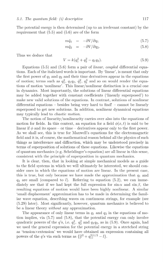
The potential energy is then determined (up to an irrelevant constant) by the
requirement that (5.5) and (5.6) are of the form
mq ¨ 1 = −∂V/∂q 1
(5.7)
mq ¨ 2 = −∂V/∂q 2 .
(5.8)
Thus we deduce that
2
2
V = k(q 1 + q 2 − q 1 q 2 ).
(5.9)
Equations (5.5) and (5.6) form a pair of linear, coupled differential equations. Each of the italicized words is important. By ‘linear’, is meant that only
the first power of q 1 and q 2 and their time derivatives appear in the equations
2
2
3
of motion; terms such as q 1 , q 1 q 2 , ˙
q 1 , q and so on would render the equa1
tions of motion ‘nonlinear’. This linear/nonlinear distinction is a crucial one
in dynamics. Most importantly, the solutions of linear differential equations
may be added together with constant coefficients (‘linearly superposed’) to
make new valid solutions of the equations. In contrast, solutions of nonlinear
differential equations – besides being very hard to find! – cannot be linearly
superposed to get new solutions. In addition, nonlinear dynamical equations
may typically lead to chaotic motion.
The notion of linearity/nonlinearity carries over also into the equations of
motion for fields. In this context, an equation for a field φ(x, t) is said to be
linear if φ and its space – or time – derivatives appear only to the first power.
As we shall see, this is true for Maxwell’s equations for the electromagnetic
field and it is, of course, the mathematical reason behind all the physics of such
things as interference and diffraction, which may be understood precisely in
terms of superposition of solutions of these equations. Likewise the equations
of quantum mechanics (e.g. Schr¨ odinger’s equation) are all linear in this sense,
consistent with the principle of superposition in quantum mechanics.
It is clear, then, that in looking at simple mechanical models as a guide
to the field systems in which we will ultimately be interested, we should consider ones in which the equations of motion are linear. In the present case,
this is true, but only because we have made the approximation that q 1 and
q 2 are small (compared to l). Referring to equation (5.2), we can immediately see that if we had kept the full expression for sin α and sin β, the
resulting equations of motion would have been highly nonlinear. A similar
‘small displacement’ approximation has to be made in determining the familiar wave equation, describing waves on continuous strings, for example (see
(5.29) later). Most significantly, however, quantum mechanics is believed to
be a linear theory without any approximation.
The appearance of only linear terms in q 1 and q 2 in the equations of motion implies, via (5.7) and (5.8), that the potential energy can only involve
2
2
quadratic powers of the q’s, i.e. q 1 , q and q 1 q 2 , as in (5.9). Once again, had
2
we used the general expression for the potential energy in a stretched string
as ‘tension×extension’ we would have obtained an expression containing all
powers of the q’s via such terms as {[l
2 + q 1
2 ]
1/2
− l}.
5.1. The quantum field: (i) descriptive
The potential energy is then determined (up to an irrelevant constant) by the
requirement that (5.5) and (5.6) are of the form
mq ¨ 1 = −∂V/∂q 1
(5.7)
mq ¨ 2 = −∂V/∂q 2 .
(5.8)
Thus we deduce that
2
2
V = k(q 1 + q 2 − q 1 q 2 ).
(5.9)
Equations (5.5) and (5.6) form a pair of linear, coupled differential equations. Each of the italicized words is important. By ‘linear’, is meant that only
the first power of q 1 and q 2 and their time derivatives appear in the equations
2
2
3
of motion; terms such as q 1 , q 1 q 2 , ˙
q 1 , q and so on would render the equa1
tions of motion ‘nonlinear’. This linear/nonlinear distinction is a crucial one
in dynamics. Most importantly, the solutions of linear differential equations
may be added together with constant coefficients (‘linearly superposed’) to
make new valid solutions of the equations. In contrast, solutions of nonlinear
differential equations – besides being very hard to find! – cannot be linearly
superposed to get new solutions. In addition, nonlinear dynamical equations
may typically lead to chaotic motion.
The notion of linearity/nonlinearity carries over also into the equations of
motion for fields. In this context, an equation for a field φ(x, t) is said to be
linear if φ and its space – or time – derivatives appear only to the first power.
As we shall see, this is true for Maxwell’s equations for the electromagnetic
field and it is, of course, the mathematical reason behind all the physics of such
things as interference and diffraction, which may be understood precisely in
terms of superposition of solutions of these equations. Likewise the equations
of quantum mechanics (e.g. Schr¨ odinger’s equation) are all linear in this sense,
consistent with the principle of superposition in quantum mechanics.
It is clear, then, that in looking at simple mechanical models as a guide
to the field systems in which we will ultimately be interested, we should consider ones in which the equations of motion are linear. In the present case,
this is true, but only because we have made the approximation that q 1 and
q 2 are small (compared to l). Referring to equation (5.2), we can immediately see that if we had kept the full expression for sin α and sin β, the
resulting equations of motion would have been highly nonlinear. A similar
‘small displacement’ approximation has to be made in determining the familiar wave equation, describing waves on continuous strings, for example (see
(5.29) later). Most significantly, however, quantum mechanics is believed to
be a linear theory without any approximation.
The appearance of only linear terms in q 1 and q 2 in the equations of motion implies, via (5.7) and (5.8), that the potential energy can only involve
2
2
quadratic powers of the q’s, i.e. q 1 , q and q 1 q 2 , as in (5.9). Once again, had
2
we used the general expression for the potential energy in a stretched string
as ‘tension×extension’ we would have obtained an expression containing all
powers of the q’s via such terms as {[l
2 + q 1
2 ]
1/2
− l}.