

106
4. Lorentz Transformations and Discrete Symmetries
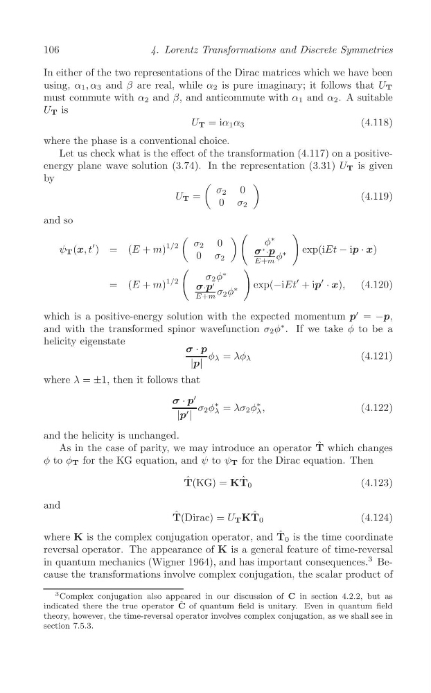
In either of the two representations of the Dirac matrices which we have been
using, α 1 , α 3 and β are real, while α 2 is pure imaginary; it follows that U T
must commute with α 2 and β, and anticommute with α 1 and α 2 . A suitable
U T is
U T = iα 1 α 3
(4.118)
where the phase is a conventional choice.
Let us check what is the effect of the transformation (4.117) on a positiveenergy plane wave solution (3.74). In the representation (3.31) U T is given
by
U T =
(
σ 2
0
0
σ 2
)
(4.119)
and so
(
) (
)
φ
∗
0
ψ T (x, t
′ ) = (E + m)
1/2
σ
0
2
σ
∗ ·p φ
∗
exp(iEt − ip · x)
σ 2
E+m
(
)
σ 2 φ
∗
′
= (E + m)
1/2
σ·p
'
exp(−iEt
′ + ip · x),
(4.120)
σ 2 φ
∗
E+m
′
which is a positive-energy solution with the expected momentum p = −p,
and with the transformed spinor wavefunction σ 2 φ
∗ . If we take φ to be a
helicity eigenstate
σ · p φ λ = λφ λ
(4.121)
|p|
where λ = ±1, then it follows that
′
σ · p σ 2 φ
∗ = λσ 2 φ
∗
λ ,
(4.122)
λ
|p ′ |
and the helicity is unchanged.
As in the case of parity, we may introduce an operator T ˆ which changes
φ to φ T for the KG equation, and ψ to ψ T for the Dirac equation. Then
T ˆ (KG) = KT ˆ 0
(4.123)
and
ˆ
U T K ˆ
T(Dirac) =
T 0
(4.124)
where K is the complex conjugation operator, and T ˆ 0 is the time coordinate
reversal operator. The appearance of K is a general feature of time-reversal
3
in quantum mechanics (Wigner 1964), and has important consequences. Because the transformations involve complex conjugation, the scalar product of
3 Complex conjugation also appeared in our discussion of C in section 4.2.2, but as
indicated there the true operator C of quantum field is unitary. Even in quantum field
ˆ
theory, however, the time-reversal operator involves complex conjugation, as we shall see in
section 7.5.3.
4. Lorentz Transformations and Discrete Symmetries
In either of the two representations of the Dirac matrices which we have been
using, α 1 , α 3 and β are real, while α 2 is pure imaginary; it follows that U T
must commute with α 2 and β, and anticommute with α 1 and α 2 . A suitable
U T is
U T = iα 1 α 3
(4.118)
where the phase is a conventional choice.
Let us check what is the effect of the transformation (4.117) on a positiveenergy plane wave solution (3.74). In the representation (3.31) U T is given
by
U T =
(
σ 2
0
0
σ 2
)
(4.119)
and so
(
) (
)
φ
∗
0
ψ T (x, t
′ ) = (E + m)
1/2
σ
0
2
σ
∗ ·p φ
∗
exp(iEt − ip · x)
σ 2
E+m
(
)
σ 2 φ
∗
′
= (E + m)
1/2
σ·p
'
exp(−iEt
′ + ip · x),
(4.120)
σ 2 φ
∗
E+m
′
which is a positive-energy solution with the expected momentum p = −p,
and with the transformed spinor wavefunction σ 2 φ
∗ . If we take φ to be a
helicity eigenstate
σ · p φ λ = λφ λ
(4.121)
|p|
where λ = ±1, then it follows that
′
σ · p σ 2 φ
∗ = λσ 2 φ
∗
λ ,
(4.122)
λ
|p ′ |
and the helicity is unchanged.
As in the case of parity, we may introduce an operator T ˆ which changes
φ to φ T for the KG equation, and ψ to ψ T for the Dirac equation. Then
T ˆ (KG) = KT ˆ 0
(4.123)
and
ˆ
U T K ˆ
T(Dirac) =
T 0
(4.124)
where K is the complex conjugation operator, and T ˆ 0 is the time coordinate
reversal operator. The appearance of K is a general feature of time-reversal
3
in quantum mechanics (Wigner 1964), and has important consequences. Because the transformations involve complex conjugation, the scalar product of
3 Complex conjugation also appeared in our discussion of C in section 4.2.2, but as
indicated there the true operator C of quantum field is unitary. Even in quantum field
ˆ
theory, however, the time-reversal operator involves complex conjugation, as we shall see in
section 7.5.3.