

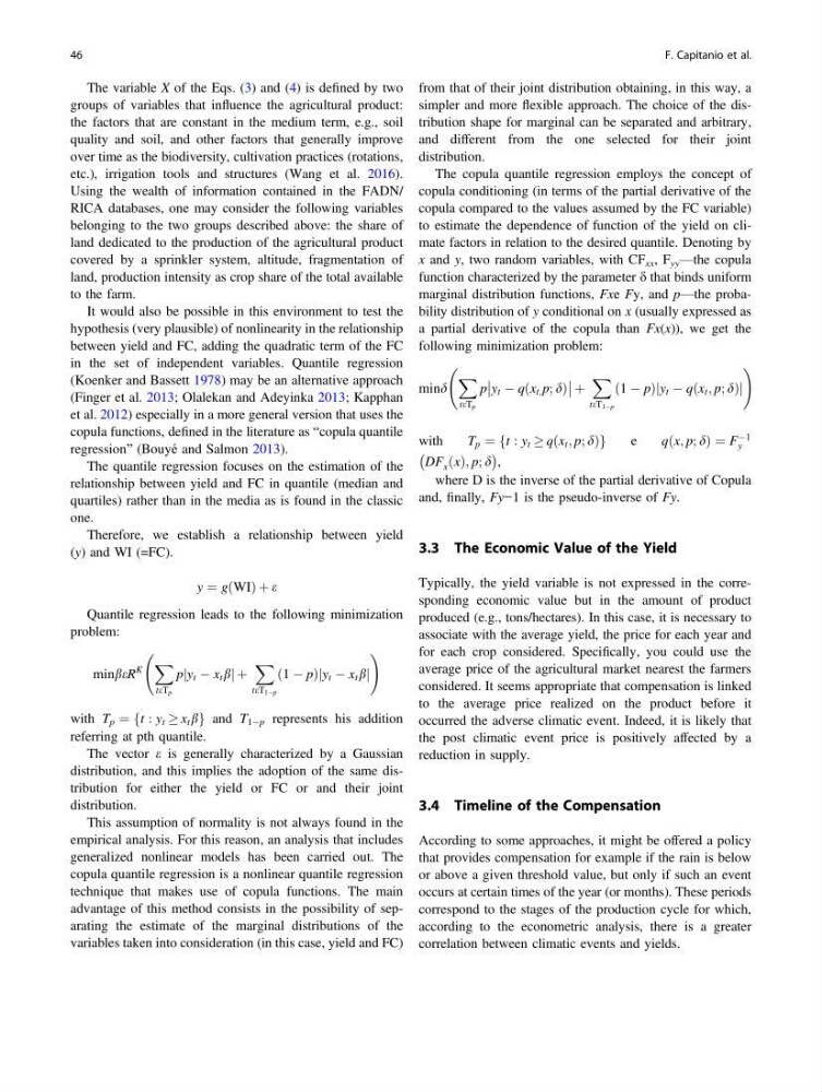
The variable X of the Eqs. (3) and (4) is defined by two
groups of variables that influence the agricultural product:
the factors that are constant in the medium term, e.g., soil
quality and soil, and other factors that generally improve
over time as the biodiversity, cultivation practices (rotations,
etc.), irrigation tools and structures (Wang et al. 2016).
Using the wealth of information contained in the FADN/
RICA databases, one may consider the following variables
belonging to the two groups described above: the share of
land dedicated to the production of the agricultural product
covered by a sprinkler system, altitude, fragmentation of
land, production intensity as crop share of the total available
to the farm.
It would also be possible in this environment to test the
hypothesis (very plausible) of nonlinearity in the relationship
between yield and FC, adding the quadratic term of the FC
in the set of independent variables. Quantile regression
(Koenker and Bassett 1978) may be an alternative approach
(Finger et al. 2013; Olalekan and Adeyinka 2013; Kapphan
et al. 2012) especially in a more general version that uses the
copula functions, defined in the literature as “copula quantile
regression” (Bouyé and Salmon 2013).
The quantile regression focuses on the estimation of the
relationship between yield and FC in quantile (median and
quartiles) rather than in the media as is found in the classic
one.
Therefore, we establish a relationship between yield
(y) and WI (=FC).
y ¼ gðWIÞ þ e
Quantile regression leads to the following minimization
problem:
minbeR
K
X
teT p
p y t À x t b
j
jþ
X
teT 1Àp
ð1 À pÞ y t À x t b
j
j
!
with T p ¼ t : y t ! x t b
f
g and T 1Àp represents his addition
referring at pth quantile.
The vector e is generally characterized by a Gaussian
distribution, and this implies the adoption of the same distribution for either the yield or FC or and their joint
distribution.
This assumption of normality is not always found in the
empirical analysis. For this reason, an analysis that includes
generalized nonlinear models has been carried out. The
copula quantile regression is a nonlinear quantile regression
technique that makes use of copula functions. The main
advantage of this method consists in the possibility of separating the estimate of the marginal distributions of the
variables taken into consideration (in this case, yield and FC)
from that of their joint distribution obtaining, in this way, a
simpler and more flexible approach. The choice of the distribution shape for marginal can be separated and arbitrary,
and different from the one selected for their joint
distribution.
The copula quantile regression employs the concept of
copula conditioning (in terms of the partial derivative of the
copula compared to the values assumed by the FC variable)
to estimate the dependence of function of the yield on climate factors in relation to the desired quantile. Denoting by
x and y, two random variables, with CF xx , F yy —the copula
function characterized by the parameter d that binds uniform
marginal distribution functions, Fxe Fy, and p—the probability distribution of y conditional on x (usually expressed as
a partial derivative of the copula than Fx(x)), we get the
following minimization problem:
mind
X
teT p
p y t À qðx t; p; dÞ
þ
X
teT 1Àp
ð1 À pÞ y t À qðx t ; p; dÞ
j
j
!
with
T p ¼ t : y t ! qðx t ; p; dÞ
f
g
e
q x; p; d
ð
Þ¼F
À1
y
DF x x
ð Þ; p; d
À
Á
,
where D is the inverse of the partial derivative of Copula
and, finally, Fy−1 is the pseudo-inverse of Fy.
3.3 The Economic Value of the Yield
Typically, the yield variable is not expressed in the corresponding economic value but in the amount of product
produced (e.g., tons/hectares). In this case, it is necessary to
associate with the average yield, the price for each year and
for each crop considered. Specifically, you could use the
average price of the agricultural market nearest the farmers
considered. It seems appropriate that compensation is linked
to the average price realized on the product before it
occurred the adverse climatic event. Indeed, it is likely that
the post climatic event price is positively affected by a
reduction in supply.
3.4 Timeline of the Compensation
According to some approaches, it might be offered a policy
that provides compensation for example if the rain is below
or above a given threshold value, but only if such an event
occurs at certain times of the year (or months). These periods
correspond to the stages of the production cycle for which,
according to the econometric analysis, there is a greater
correlation between climatic events and yields.
46
F. Capitanio et al.
groups of variables that influence the agricultural product:
the factors that are constant in the medium term, e.g., soil
quality and soil, and other factors that generally improve
over time as the biodiversity, cultivation practices (rotations,
etc.), irrigation tools and structures (Wang et al. 2016).
Using the wealth of information contained in the FADN/
RICA databases, one may consider the following variables
belonging to the two groups described above: the share of
land dedicated to the production of the agricultural product
covered by a sprinkler system, altitude, fragmentation of
land, production intensity as crop share of the total available
to the farm.
It would also be possible in this environment to test the
hypothesis (very plausible) of nonlinearity in the relationship
between yield and FC, adding the quadratic term of the FC
in the set of independent variables. Quantile regression
(Koenker and Bassett 1978) may be an alternative approach
(Finger et al. 2013; Olalekan and Adeyinka 2013; Kapphan
et al. 2012) especially in a more general version that uses the
copula functions, defined in the literature as “copula quantile
regression” (Bouyé and Salmon 2013).
The quantile regression focuses on the estimation of the
relationship between yield and FC in quantile (median and
quartiles) rather than in the media as is found in the classic
one.
Therefore, we establish a relationship between yield
(y) and WI (=FC).
y ¼ gðWIÞ þ e
Quantile regression leads to the following minimization
problem:
minbeR
K
X
teT p
p y t À x t b
j
jþ
X
teT 1Àp
ð1 À pÞ y t À x t b
j
j
!
with T p ¼ t : y t ! x t b
f
g and T 1Àp represents his addition
referring at pth quantile.
The vector e is generally characterized by a Gaussian
distribution, and this implies the adoption of the same distribution for either the yield or FC or and their joint
distribution.
This assumption of normality is not always found in the
empirical analysis. For this reason, an analysis that includes
generalized nonlinear models has been carried out. The
copula quantile regression is a nonlinear quantile regression
technique that makes use of copula functions. The main
advantage of this method consists in the possibility of separating the estimate of the marginal distributions of the
variables taken into consideration (in this case, yield and FC)
from that of their joint distribution obtaining, in this way, a
simpler and more flexible approach. The choice of the distribution shape for marginal can be separated and arbitrary,
and different from the one selected for their joint
distribution.
The copula quantile regression employs the concept of
copula conditioning (in terms of the partial derivative of the
copula compared to the values assumed by the FC variable)
to estimate the dependence of function of the yield on climate factors in relation to the desired quantile. Denoting by
x and y, two random variables, with CF xx , F yy —the copula
function characterized by the parameter d that binds uniform
marginal distribution functions, Fxe Fy, and p—the probability distribution of y conditional on x (usually expressed as
a partial derivative of the copula than Fx(x)), we get the
following minimization problem:
mind
X
teT p
p y t À qðx t; p; dÞ
þ
X
teT 1Àp
ð1 À pÞ y t À qðx t ; p; dÞ
j
j
!
with
T p ¼ t : y t ! qðx t ; p; dÞ
f
g
e
q x; p; d
ð
Þ¼F
À1
y
DF x x
ð Þ; p; d
À
Á
,
where D is the inverse of the partial derivative of Copula
and, finally, Fy−1 is the pseudo-inverse of Fy.
3.3 The Economic Value of the Yield
Typically, the yield variable is not expressed in the corresponding economic value but in the amount of product
produced (e.g., tons/hectares). In this case, it is necessary to
associate with the average yield, the price for each year and
for each crop considered. Specifically, you could use the
average price of the agricultural market nearest the farmers
considered. It seems appropriate that compensation is linked
to the average price realized on the product before it
occurred the adverse climatic event. Indeed, it is likely that
the post climatic event price is positively affected by a
reduction in supply.
3.4 Timeline of the Compensation
According to some approaches, it might be offered a policy
that provides compensation for example if the rain is below
or above a given threshold value, but only if such an event
occurs at certain times of the year (or months). These periods
correspond to the stages of the production cycle for which,
according to the econometric analysis, there is a greater
correlation between climatic events and yields.
46
F. Capitanio et al.