

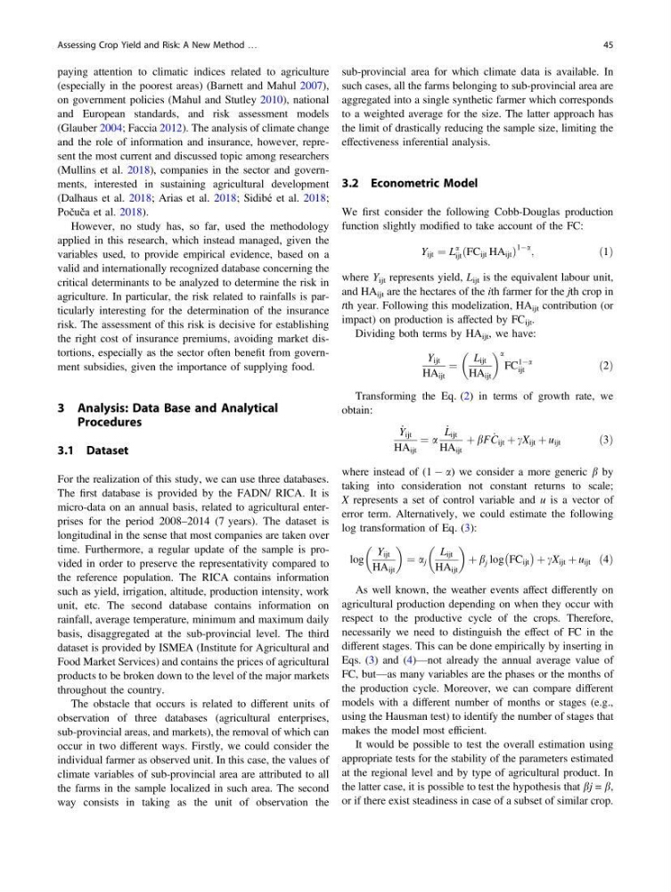
paying attention to climatic indices related to agriculture
(especially in the poorest areas) (Barnett and Mahul 2007),
on government policies (Mahul and Stutley 2010), national
and European standards, and risk assessment models
(Glauber 2004; Faccia 2012). The analysis of climate change
and the role of information and insurance, however, represent the most current and discussed topic among researchers
(Mullins et al. 2018), companies in the sector and governments, interested in sustaining agricultural development
(Dalhaus et al. 2018; Arias et al. 2018; Sidibé et al. 2018;
Počuča et al. 2018).
However, no study has, so far, used the methodology
applied in this research, which instead managed, given the
variables used, to provide empirical evidence, based on a
valid and internationally recognized database concerning the
critical determinants to be analyzed to determine the risk in
agriculture. In particular, the risk related to rainfalls is particularly interesting for the determination of the insurance
risk. The assessment of this risk is decisive for establishing
the right cost of insurance premiums, avoiding market distortions, especially as the sector often benefit from government subsidies, given the importance of supplying food.
3 Analysis: Data Base and Analytical
Procedures
3.1 Dataset
For the realization of this study, we can use three databases.
The first database is provided by the FADN/ RICA. It is
micro-data on an annual basis, related to agricultural enterprises for the period 2008–2014 (7 years). The dataset is
longitudinal in the sense that most companies are taken over
time. Furthermore, a regular update of the sample is provided in order to preserve the representativity compared to
the reference population. The RICA contains information
such as yield, irrigation, altitude, production intensity, work
unit, etc. The second database contains information on
rainfall, average temperature, minimum and maximum daily
basis, disaggregated at the sub-provincial level. The third
dataset is provided by ISMEA (Institute for Agricultural and
Food Market Services) and contains the prices of agricultural
products to be broken down to the level of the major markets
throughout the country.
The obstacle that occurs is related to different units of
observation of three databases (agricultural enterprises,
sub-provincial areas, and markets), the removal of which can
occur in two different ways. Firstly, we could consider the
individual farmer as observed unit. In this case, the values of
climate variables of sub-provincial area are attributed to all
the farms in the sample localized in such area. The second
way consists in taking as the unit of observation the
sub-provincial area for which climate data is available. In
such cases, all the farms belonging to sub-provincial area are
aggregated into a single synthetic farmer which corresponds
to a weighted average for the size. The latter approach has
the limit of drastically reducing the sample size, limiting the
effectiveness inferential analysis.
3.2 Econometric Model
We first consider the following Cobb-Douglas production
function slightly modified to take account of the FC:
Y ijt ¼ L
a
ijt ðFC ijt HA ijt Þ
1Àa ;
ð1Þ
where Y ijt represents yield, L ijt is the equivalent labour unit,
and HA ijt are the hectares of the ith farmer for the jth crop in
tth year. Following this modelization, HA ijt contribution (or
impact) on production is affected by FC ijt .
Dividing both terms by HA ijt , we have:
Y ijt
HA ijt
¼
L ijt
HA ijt
a
FC
1Àa
ijt
ð2Þ
Transforming the Eq. (2) in terms of growth rate, we
obtain:
_
Y ijt
HA ijt
¼ a
_
L ijt
HA ijt
þ bF _
C ijt þ cX ijt þ u ijt
ð3Þ
where instead of (1 À a) we consider a more generic b by
taking into consideration not constant returns to scale;
X represents a set of control variable and u is a vector of
error term. Alternatively, we could estimate the following
log transformation of Eq. (3):
log
Y ijt
HA ijt
¼ a j
L ijt
HA ijt
þ b j log FC ijt
À
Á þ cX ijt þ u ijt ð4Þ
As well known, the weather events affect differently on
agricultural production depending on when they occur with
respect to the productive cycle of the crops. Therefore,
necessarily we need to distinguish the effect of FC in the
different stages. This can be done empirically by inserting in
Eqs. (3) and (4)—not already the annual average value of
FC, but—as many variables are the phases or the months of
the production cycle. Moreover, we can compare different
models with a different number of months or stages (e.g.,
using the Hausman test) to identify the number of stages that
makes the model most efficient.
It would be possible to test the overall estimation using
appropriate tests for the stability of the parameters estimated
at the regional level and by type of agricultural product. In
the latter case, it is possible to test the hypothesis that bj = b,
or if there exist steadiness in case of a subset of similar crop.
Assessing Crop Yield and Risk: A New Method …
45
(especially in the poorest areas) (Barnett and Mahul 2007),
on government policies (Mahul and Stutley 2010), national
and European standards, and risk assessment models
(Glauber 2004; Faccia 2012). The analysis of climate change
and the role of information and insurance, however, represent the most current and discussed topic among researchers
(Mullins et al. 2018), companies in the sector and governments, interested in sustaining agricultural development
(Dalhaus et al. 2018; Arias et al. 2018; Sidibé et al. 2018;
Počuča et al. 2018).
However, no study has, so far, used the methodology
applied in this research, which instead managed, given the
variables used, to provide empirical evidence, based on a
valid and internationally recognized database concerning the
critical determinants to be analyzed to determine the risk in
agriculture. In particular, the risk related to rainfalls is particularly interesting for the determination of the insurance
risk. The assessment of this risk is decisive for establishing
the right cost of insurance premiums, avoiding market distortions, especially as the sector often benefit from government subsidies, given the importance of supplying food.
3 Analysis: Data Base and Analytical
Procedures
3.1 Dataset
For the realization of this study, we can use three databases.
The first database is provided by the FADN/ RICA. It is
micro-data on an annual basis, related to agricultural enterprises for the period 2008–2014 (7 years). The dataset is
longitudinal in the sense that most companies are taken over
time. Furthermore, a regular update of the sample is provided in order to preserve the representativity compared to
the reference population. The RICA contains information
such as yield, irrigation, altitude, production intensity, work
unit, etc. The second database contains information on
rainfall, average temperature, minimum and maximum daily
basis, disaggregated at the sub-provincial level. The third
dataset is provided by ISMEA (Institute for Agricultural and
Food Market Services) and contains the prices of agricultural
products to be broken down to the level of the major markets
throughout the country.
The obstacle that occurs is related to different units of
observation of three databases (agricultural enterprises,
sub-provincial areas, and markets), the removal of which can
occur in two different ways. Firstly, we could consider the
individual farmer as observed unit. In this case, the values of
climate variables of sub-provincial area are attributed to all
the farms in the sample localized in such area. The second
way consists in taking as the unit of observation the
sub-provincial area for which climate data is available. In
such cases, all the farms belonging to sub-provincial area are
aggregated into a single synthetic farmer which corresponds
to a weighted average for the size. The latter approach has
the limit of drastically reducing the sample size, limiting the
effectiveness inferential analysis.
3.2 Econometric Model
We first consider the following Cobb-Douglas production
function slightly modified to take account of the FC:
Y ijt ¼ L
a
ijt ðFC ijt HA ijt Þ
1Àa ;
ð1Þ
where Y ijt represents yield, L ijt is the equivalent labour unit,
and HA ijt are the hectares of the ith farmer for the jth crop in
tth year. Following this modelization, HA ijt contribution (or
impact) on production is affected by FC ijt .
Dividing both terms by HA ijt , we have:
Y ijt
HA ijt
¼
L ijt
HA ijt
a
FC
1Àa
ijt
ð2Þ
Transforming the Eq. (2) in terms of growth rate, we
obtain:
_
Y ijt
HA ijt
¼ a
_
L ijt
HA ijt
þ bF _
C ijt þ cX ijt þ u ijt
ð3Þ
where instead of (1 À a) we consider a more generic b by
taking into consideration not constant returns to scale;
X represents a set of control variable and u is a vector of
error term. Alternatively, we could estimate the following
log transformation of Eq. (3):
log
Y ijt
HA ijt
¼ a j
L ijt
HA ijt
þ b j log FC ijt
À
Á þ cX ijt þ u ijt ð4Þ
As well known, the weather events affect differently on
agricultural production depending on when they occur with
respect to the productive cycle of the crops. Therefore,
necessarily we need to distinguish the effect of FC in the
different stages. This can be done empirically by inserting in
Eqs. (3) and (4)—not already the annual average value of
FC, but—as many variables are the phases or the months of
the production cycle. Moreover, we can compare different
models with a different number of months or stages (e.g.,
using the Hausman test) to identify the number of stages that
makes the model most efficient.
It would be possible to test the overall estimation using
appropriate tests for the stability of the parameters estimated
at the regional level and by type of agricultural product. In
the latter case, it is possible to test the hypothesis that bj = b,
or if there exist steadiness in case of a subset of similar crop.
Assessing Crop Yield and Risk: A New Method …
45