

54
3 Principle and Practice of Three-Dimensional Transmission …
I = I 0 exp
⎛
⎝ −
l
f (x, y)dL
⎞
⎠
(3.1)
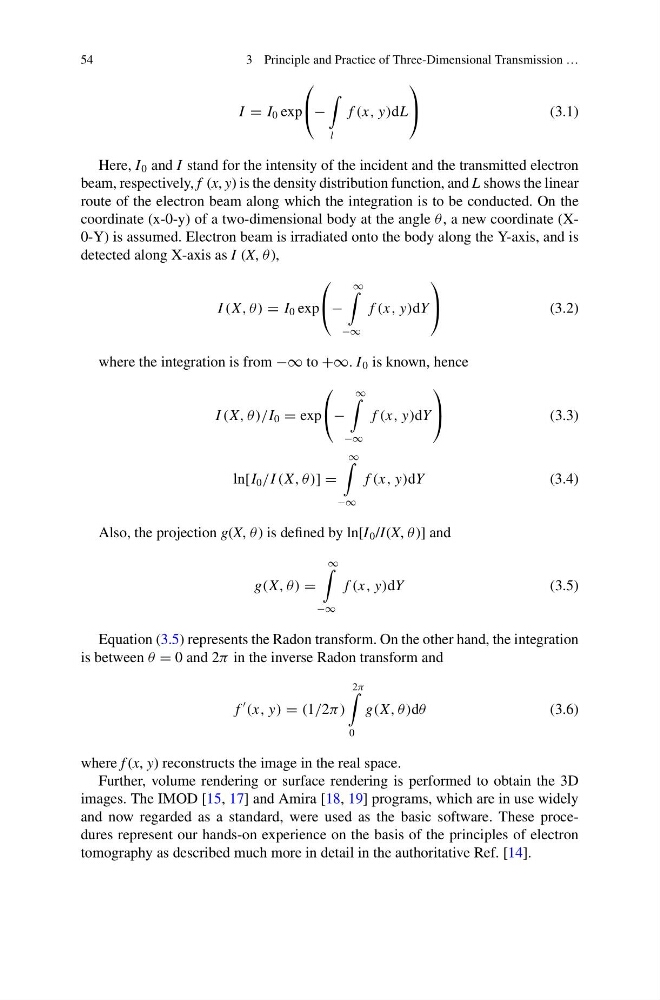
Here, I 0 and I stand for the intensity of the incident and the transmitted electron
beam, respectively, f (x, y) is the density distribution function, and L shows the linear
route of the electron beam along which the integration is to be conducted. On the
coordinate (x-0-y) of a two-dimensional body at the angle θ , a new coordinate (X0-Y) is assumed. Electron beam is irradiated onto the body along the Y-axis, and is
detected along X-axis as I (X, θ ),
I (X, θ) = I 0 exp
⎛
⎝ −
∞
−∞
f (x, y)dY
⎞
⎠
(3.2)
where the integration is from −∞ to +∞. I 0 is known, hence
I (X, θ)/I 0 = exp
⎛
⎝ −
∞
−∞
f (x, y)dY
⎞
⎠
(3.3)
ln[I 0 /I (X, θ)] =
∞
−∞
f (x, y)dY
(3.4)
Also, the projection g(X, θ ) is defined by ln[I 0 /I(X, θ )] and
g(X, θ) =
∞
−∞
f (x, y)dY
(3.5)
Equation (3.5) represents the Radon transform. On the other hand, the integration
is between θ = 0 and 2π in the inverse Radon transform and
f
(x, y) = (1/2π)
2π
0
g(X, θ)dθ
(3.6)
where f (x, y) reconstructs the image in the real space.
Further, volume rendering or surface rendering is performed to obtain the 3D
images. The IMOD [15, 17] and Amira [18, 19] programs, which are in use widely
and now regarded as a standard, were used as the basic software. These procedures represent our hands-on experience on the basis of the principles of electron
tomography as described much more in detail in the authoritative Ref. [14].
3 Principle and Practice of Three-Dimensional Transmission …
I = I 0 exp
⎛
⎝ −
l
f (x, y)dL
⎞
⎠
(3.1)
Here, I 0 and I stand for the intensity of the incident and the transmitted electron
beam, respectively, f (x, y) is the density distribution function, and L shows the linear
route of the electron beam along which the integration is to be conducted. On the
coordinate (x-0-y) of a two-dimensional body at the angle θ , a new coordinate (X0-Y) is assumed. Electron beam is irradiated onto the body along the Y-axis, and is
detected along X-axis as I (X, θ ),
I (X, θ) = I 0 exp
⎛
⎝ −
∞
−∞
f (x, y)dY
⎞
⎠
(3.2)
where the integration is from −∞ to +∞. I 0 is known, hence
I (X, θ)/I 0 = exp
⎛
⎝ −
∞
−∞
f (x, y)dY
⎞
⎠
(3.3)
ln[I 0 /I (X, θ)] =
∞
−∞
f (x, y)dY
(3.4)
Also, the projection g(X, θ ) is defined by ln[I 0 /I(X, θ )] and
g(X, θ) =
∞
−∞
f (x, y)dY
(3.5)
Equation (3.5) represents the Radon transform. On the other hand, the integration
is between θ = 0 and 2π in the inverse Radon transform and
f
(x, y) = (1/2π)
2π
0
g(X, θ)dθ
(3.6)
where f (x, y) reconstructs the image in the real space.
Further, volume rendering or surface rendering is performed to obtain the 3D
images. The IMOD [15, 17] and Amira [18, 19] programs, which are in use widely
and now regarded as a standard, were used as the basic software. These procedures represent our hands-on experience on the basis of the principles of electron
tomography as described much more in detail in the authoritative Ref. [14].