

sufficiently diluted in solution to not interact from each other. The solvent contribution is treated as an independent parameter uncoupled to the chain contribution,
while it is the necessary vector of transfer of the stress from and to the substrate.
The chain is seen as a succession of freely joined elastic springs. Each spring
represents a group of monomers (blob) unperturbed by others (Gaussian statistics).
In this frame, the generalized Maxwell model can be applied, and the viscoelastic
curve is assimilated to it:
G
0
ω
ð Þ ¼ nkT
X Z
p¼1
ω
2
τ
2
p
1 þ ω 2 :τ 2
p
G
00
ω
ð Þ ¼ ω:η s þ n:kT
X Z
p¼1
ω:τ p
1 þ ω 2 :τ 2
p
where G
0 (ω) and G
00 (ω) are the shear elastic modulus and the viscous modulus,
respectively, η s is the solvent viscosity, τ p is the relaxation time of the group p, Z is
the number of springs, n is the number of chain per volume unit, and T is the
temperature. At low frequency, G
0 scales as ω
2 with a zero-frequency limit
corresponding to the absence of shear elastic component. The zero-frequency limit
of the viscous part gives also rise to a collapse (G
00
ffi 0). The viscoelastic model for
fluids predicts neither shear elasticity nor viscous modulus at the zero-frequency
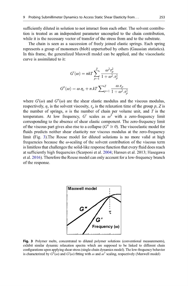
limit (Fig. 3).The Rouse model for diluted solutions is no more valid at high
frequencies because the ω-scaling of the solvent contribution of the viscous term
is limitless that challenges the solid-like response function that every fluid does reach
at sufficiently high frequencies (Scarponi et al. 2004; Hansen et al. 2013; Hasegawa
et al. 2016). Therefore the Rouse model can only account for a low-frequency branch
of the response.
Fig. 3 Polymer melts, concentrated to diluted polymer solutions (conventional measurements),
exhibit similar dynamic relaxation spectra which are supposed to be linked to different chain
configurations upon applying shear stress (single-chain dynamics model). The low-frequency behavior
is characterized by G
00 (ω) and G
0 (ω) fitting with ω and ω
2 scaling, respectively (Maxwell model)
9 Probing Submillimeter Dynamics to Access Static Shear Elasticity from. . .
253
while it is the necessary vector of transfer of the stress from and to the substrate.
The chain is seen as a succession of freely joined elastic springs. Each spring
represents a group of monomers (blob) unperturbed by others (Gaussian statistics).
In this frame, the generalized Maxwell model can be applied, and the viscoelastic
curve is assimilated to it:
G
0
ω
ð Þ ¼ nkT
X Z
p¼1
ω
2
τ
2
p
1 þ ω 2 :τ 2
p
G
00
ω
ð Þ ¼ ω:η s þ n:kT
X Z
p¼1
ω:τ p
1 þ ω 2 :τ 2
p
where G
0 (ω) and G
00 (ω) are the shear elastic modulus and the viscous modulus,
respectively, η s is the solvent viscosity, τ p is the relaxation time of the group p, Z is
the number of springs, n is the number of chain per volume unit, and T is the
temperature. At low frequency, G
0 scales as ω
2 with a zero-frequency limit
corresponding to the absence of shear elastic component. The zero-frequency limit
of the viscous part gives also rise to a collapse (G
00
ffi 0). The viscoelastic model for
fluids predicts neither shear elasticity nor viscous modulus at the zero-frequency
limit (Fig. 3).The Rouse model for diluted solutions is no more valid at high
frequencies because the ω-scaling of the solvent contribution of the viscous term
is limitless that challenges the solid-like response function that every fluid does reach
at sufficiently high frequencies (Scarponi et al. 2004; Hansen et al. 2013; Hasegawa
et al. 2016). Therefore the Rouse model can only account for a low-frequency branch
of the response.
Fig. 3 Polymer melts, concentrated to diluted polymer solutions (conventional measurements),
exhibit similar dynamic relaxation spectra which are supposed to be linked to different chain
configurations upon applying shear stress (single-chain dynamics model). The low-frequency behavior
is characterized by G
00 (ω) and G
0 (ω) fitting with ω and ω
2 scaling, respectively (Maxwell model)
9 Probing Submillimeter Dynamics to Access Static Shear Elasticity from. . .
253