

57 Comparison of the Performance of AERMOD …
361
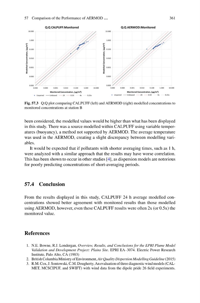
Fig. 57.3 Q:Q plot comparing CALPUFF (left) and AERMOD (right) modelled concentrations to
monitored concentrations at station B
been considered, the modelled values would be higher than what has been displayed
in this study. There was a source modelled within CALPUFF using variable temperatures (buoyancy), a method not supported by AERMOD. The average temperature
was used in the AERMOD, creating a slight discrepancy between modelling variables.
It would be expected that if pollutants with shorter averaging times, such as 1 h,
were analyzed with a similar approach that the results may have worse correlation.
This has been shown to occur in other studies [4], as dispersion models are notorious
for poorly predicting concentrations of short-averaging periods.
57.4 Conclusion
From the results displayed in this study, CALPUFF 24 h average modelled concentrations showed better agreement with monitored results than those modelled
using AERMOD, however, even these CALPUFF results were often 2x (or 0.5x) the
monitored value.
References
1. N.E. Bowne, R.J. Londergan, Overview, Results, and Conclusions for the EPRI Plume Model
Validation and Development Project: Plains Site. EPRI EA–3074. Electric Power Research
Institute, Palo Alto, CA (1983)
2. British Columbia Ministry of Environment, Air Quality Dispersion Modelling Guideline (2015)
3. R.M. Cox, J. Sontowski, C.M. Dougherty, An evaluation of three diagnostic wind models (CALMET, MCSCIPUF, and SWIFT) with wind data from the dipole pride 26 field experiments.
361
Fig. 57.3 Q:Q plot comparing CALPUFF (left) and AERMOD (right) modelled concentrations to
monitored concentrations at station B
been considered, the modelled values would be higher than what has been displayed
in this study. There was a source modelled within CALPUFF using variable temperatures (buoyancy), a method not supported by AERMOD. The average temperature
was used in the AERMOD, creating a slight discrepancy between modelling variables.
It would be expected that if pollutants with shorter averaging times, such as 1 h,
were analyzed with a similar approach that the results may have worse correlation.
This has been shown to occur in other studies [4], as dispersion models are notorious
for poorly predicting concentrations of short-averaging periods.
57.4 Conclusion
From the results displayed in this study, CALPUFF 24 h average modelled concentrations showed better agreement with monitored results than those modelled
using AERMOD, however, even these CALPUFF results were often 2x (or 0.5x) the
monitored value.
References
1. N.E. Bowne, R.J. Londergan, Overview, Results, and Conclusions for the EPRI Plume Model
Validation and Development Project: Plains Site. EPRI EA–3074. Electric Power Research
Institute, Palo Alto, CA (1983)
2. British Columbia Ministry of Environment, Air Quality Dispersion Modelling Guideline (2015)
3. R.M. Cox, J. Sontowski, C.M. Dougherty, An evaluation of three diagnostic wind models (CALMET, MCSCIPUF, and SWIFT) with wind data from the dipole pride 26 field experiments.