

90
P. De Meutter et al.
In this paper, we assess the possible source areas for the Ru-106 based on measurements from the International Monitoring System (IMS) for the verification of the
Comprehensive Nuclear-Test-Ban-Treaty that detected Ru-106 throughout the northern hemisphere. We use an adjoint approach and quantify meteorological uncertainty
using the ensemble approach.
15.2 Data and Methods
Meteorological data from the Integrated Forecasting System operational at ECMWF
have been used. The extracted data had horizontal grid spacings of 1
◦ and 137 nonuniform vertical levels up to 0.01 hPa. The inverse modelling was performed using
282 Ru-106 detections and non-detections from the International Monitoring System.
Inverse modelling involves finding a source term x(x, y, z, t) based on a vector
of observations y:
y = M x
(15.1)
here, M is the source-receptor-sensitivity matrix which is obtained by running the
atmospheric transport and dispersion model Flexpart [2] in backward mode [3]. Wet
deposition is taken into account. In practice, no perfect match between the observed
and simulated activity concentrations is possible, since both the source-receptorsensitivity matrix and the observations contain uncertainties. Instead, the disagreement is minimised using an optimisation procedure. A cost function is defined to
quantify the disagreement. It is assumed that the true source lies in one of the grid
boxes having the lowest cost function value. There is no need to rerun the atmospheric transport model during the optimisation: only the source term x(x, y, z, t)
needs to be varied until a sufficiently good match is found with y.
We assume that the Ru-106 detections originated from a single point source in the
lowest model level. We perform the optimisation for each grid box separately in the
lowest model level (each grid box is thus assumed to be a source; since this does not
involve rerunning the atmospheric transport and dispersion model, this procedure is
fast). The result is a cost function value for each grid box, and an associated optimal
source term. Grid boxes with a low cost function are assumed to be possible source
locations.
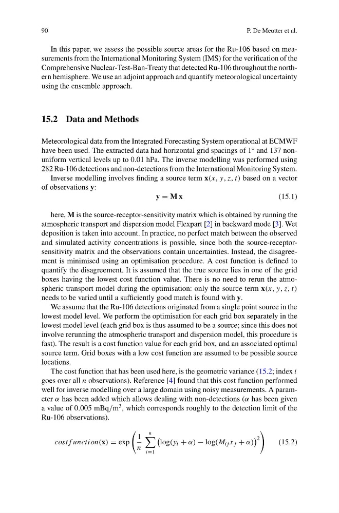
The cost function that has been used here, is the geometric variance (15.2; index i
goes over all n observations). Reference [4] found that this cost function performed
well for inverse modelling over a large domain using noisy measurements. A parameter α has been added which allows dealing with non-detections (α has been given
a value of 0.005 mBq/m
3 , which corresponds roughly to the detection limit of the
Ru-106 observations).
cost f unction(x) = exp
1
n
n
i=1
log(y i + α) − log(M i j x j + α)
2
(15.2)
P. De Meutter et al.
In this paper, we assess the possible source areas for the Ru-106 based on measurements from the International Monitoring System (IMS) for the verification of the
Comprehensive Nuclear-Test-Ban-Treaty that detected Ru-106 throughout the northern hemisphere. We use an adjoint approach and quantify meteorological uncertainty
using the ensemble approach.
15.2 Data and Methods
Meteorological data from the Integrated Forecasting System operational at ECMWF
have been used. The extracted data had horizontal grid spacings of 1
◦ and 137 nonuniform vertical levels up to 0.01 hPa. The inverse modelling was performed using
282 Ru-106 detections and non-detections from the International Monitoring System.
Inverse modelling involves finding a source term x(x, y, z, t) based on a vector
of observations y:
y = M x
(15.1)
here, M is the source-receptor-sensitivity matrix which is obtained by running the
atmospheric transport and dispersion model Flexpart [2] in backward mode [3]. Wet
deposition is taken into account. In practice, no perfect match between the observed
and simulated activity concentrations is possible, since both the source-receptorsensitivity matrix and the observations contain uncertainties. Instead, the disagreement is minimised using an optimisation procedure. A cost function is defined to
quantify the disagreement. It is assumed that the true source lies in one of the grid
boxes having the lowest cost function value. There is no need to rerun the atmospheric transport model during the optimisation: only the source term x(x, y, z, t)
needs to be varied until a sufficiently good match is found with y.
We assume that the Ru-106 detections originated from a single point source in the
lowest model level. We perform the optimisation for each grid box separately in the
lowest model level (each grid box is thus assumed to be a source; since this does not
involve rerunning the atmospheric transport and dispersion model, this procedure is
fast). The result is a cost function value for each grid box, and an associated optimal
source term. Grid boxes with a low cost function are assumed to be possible source
locations.
The cost function that has been used here, is the geometric variance (15.2; index i
goes over all n observations). Reference [4] found that this cost function performed
well for inverse modelling over a large domain using noisy measurements. A parameter α has been added which allows dealing with non-detections (α has been given
a value of 0.005 mBq/m
3 , which corresponds roughly to the detection limit of the
Ru-106 observations).
cost f unction(x) = exp
1
n
n
i=1
log(y i + α) − log(M i j x j + α)
2
(15.2)