

27.8 Examples of Building Diagrams in an Uniaxial Stressed State
365
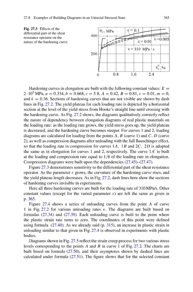
Fig. 27.3 Effects of the
differential part of the shear
resistance operator on the
nature of the hardening curve
Hardening curves in elongation are built with the following constant values: E =
2 · 10 5 MPa, a = 0.334, b = 0.668, c = 5.8, A = 0.42, B = 0.81, ε = 0.01, m = 0,
and k = 0.36. Sections of hardening curves that are not visible are shown by dash
lines in Fig. 27.2. The yield plateau for each loading rate is depicted by a horizontal
section at the level of the yield stress from Hooke’s straight line until crossing with
the hardening curve. As Fig. 27.2 shows, the diagrams qualitatively correctly reflect
the nature of dependency between elongation diagrams of real plastic materials on
the loading rate: as the loading rate grows, the yield stress goes up, the yield plateau
is decreased, and the hardening curve becomes steeper. For curves 1 and 2, loading
diagrams are calculated for loading from the points A, B (curve 1) and C, D (curve
2), as well as compression diagrams after unloading with the full Bauschinger effect,
so that the loading rate in compression for curves 1A, 1B and 2C, 2D is adopted
the same as in elongation for curves 1 and 2, respectively. The curve 1A is built
at the loading and compression rate equal to 1/6 of the loading rate in elongation.
Compression diagrams were built upon the dependencies (27.45)–(27.47).
Figure 27.3 demonstrates sensitivity to the differential part of the shear resistance
operator. As the parameter ε grows, the curvature of the hardening curve rises, and
the yield plateau length decreases. As in Fig. 27.2, dash lines here show the sections
of hardening curves invisible in experiments.
Here all three hardening curves are built for the loading rate of 310 MPa/s. Other
constant values (except for the varied parameter ε) are left the same as given in
p. 365.
Figure 27.4 shows a series of unloading curves from the point A of curve
1 in Fig. 27.2 for various unloading rates v. The diagrams are built based on
formulas (27.34) and (27.39). Each unloading curve is built to the point where
the plastic strain rate turns to zero. The coordinates of this point were defined
using formula (27.40). As we already said (p. 315), an increase in plastic strain in
unloading similar to that given in Fig. 27.4 is observed in experiments with plastic
bodies.
Diagrams shown in Fig. 27.5 reflect the strain creep process for two various stress
levels corresponding to the points A and B in curve 1 of Fig. 27.2. The charts are
built based on formula (27.50), and their asymptotes shown by dashed lines are
calculated under formula (27.51). The figure shows that for the selected constant
365
Fig. 27.3 Effects of the
differential part of the shear
resistance operator on the
nature of the hardening curve
Hardening curves in elongation are built with the following constant values: E =
2 · 10 5 MPa, a = 0.334, b = 0.668, c = 5.8, A = 0.42, B = 0.81, ε = 0.01, m = 0,
and k = 0.36. Sections of hardening curves that are not visible are shown by dash
lines in Fig. 27.2. The yield plateau for each loading rate is depicted by a horizontal
section at the level of the yield stress from Hooke’s straight line until crossing with
the hardening curve. As Fig. 27.2 shows, the diagrams qualitatively correctly reflect
the nature of dependency between elongation diagrams of real plastic materials on
the loading rate: as the loading rate grows, the yield stress goes up, the yield plateau
is decreased, and the hardening curve becomes steeper. For curves 1 and 2, loading
diagrams are calculated for loading from the points A, B (curve 1) and C, D (curve
2), as well as compression diagrams after unloading with the full Bauschinger effect,
so that the loading rate in compression for curves 1A, 1B and 2C, 2D is adopted
the same as in elongation for curves 1 and 2, respectively. The curve 1A is built
at the loading and compression rate equal to 1/6 of the loading rate in elongation.
Compression diagrams were built upon the dependencies (27.45)–(27.47).
Figure 27.3 demonstrates sensitivity to the differential part of the shear resistance
operator. As the parameter ε grows, the curvature of the hardening curve rises, and
the yield plateau length decreases. As in Fig. 27.2, dash lines here show the sections
of hardening curves invisible in experiments.
Here all three hardening curves are built for the loading rate of 310 MPa/s. Other
constant values (except for the varied parameter ε) are left the same as given in
p. 365.
Figure 27.4 shows a series of unloading curves from the point A of curve
1 in Fig. 27.2 for various unloading rates v. The diagrams are built based on
formulas (27.34) and (27.39). Each unloading curve is built to the point where
the plastic strain rate turns to zero. The coordinates of this point were defined
using formula (27.40). As we already said (p. 315), an increase in plastic strain in
unloading similar to that given in Fig. 27.4 is observed in experiments with plastic
bodies.
Diagrams shown in Fig. 27.5 reflect the strain creep process for two various stress
levels corresponding to the points A and B in curve 1 of Fig. 27.2. The charts are
built based on formula (27.50), and their asymptotes shown by dashed lines are
calculated under formula (27.51). The figure shows that for the selected constant