

15.9 Setting Boundary Problems of Plasticity Theory
211
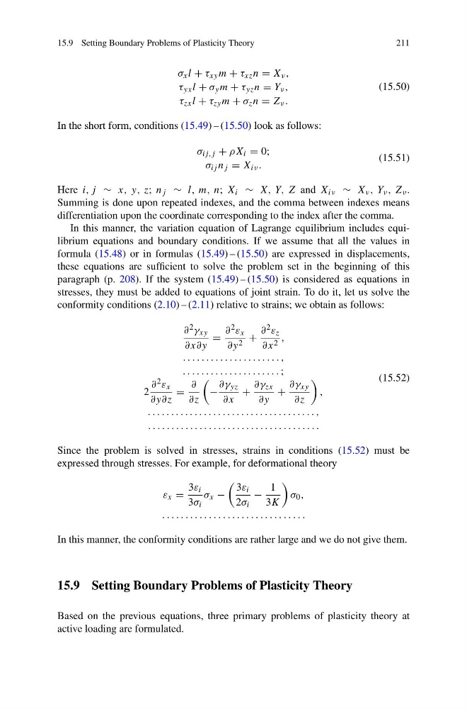
σ x l + τ xy m + τ xz n = X ν ,
τ yx l + σ y m + τ yz n = Y ν ,
τ zx l + τ zy m + σ z n = Z ν .
(15.50)
In the short form, conditions (15.49) – (15.50) look as follows:
σ ij,j + ρX i = 0;
σ ij n j = X iν .
(15.51)
Here i, j ∼ x, y, z; n j ∼ l, m, n; X i ∼ X, Y, Z and X iν ∼ X ν , Y ν , Z ν .
Summing is done upon repeated indexes, and the comma between indexes means
differentiation upon the coordinate corresponding to the index after the comma.
In this manner, the variation equation of Lagrange equilibrium includes equilibrium equations and boundary conditions. If we assume that all the values in
formula (15.48) or in formulas (15.49) – (15.50) are expressed in displacements,
these equations are sufficient to solve the problem set in the beginning of this
paragraph (p. 208). If the system (15.49) – (15.50) is considered as equations in
stresses, they must be added to equations of joint strain. To do it, let us solve the
conformity conditions (2.10) – (2.11) relative to strains; we obtain as follows:
∂ 2 γ xy
∂x∂y
=
∂ 2 ε x
∂y 2 +
∂ 2 ε z
∂x 2 ,
. . . . . . . . . . . . . . . . . . . . . ,
. . . . . . . . . . . . . . . . . . . . . ;
2
∂ 2 ε x
∂y∂z
=
∂
∂z
−
∂γ yz
∂x
+
∂γ zx
∂y
+
∂γ xy
∂z
,
. . . . . . . . . . . . . . . . . . . . . . . . . . . . . . . . . . . . ,
. . . . . . . . . . . . . . . . . . . . . . . . . . . . . . . . . . . . .
(15.52)
Since the problem is solved in stresses, strains in conditions (15.52) must be
expressed through stresses. For example, for deformational theory
ε x =
3ε i
3σ i
σ x −
3ε i
2σ i
−
1
3K
σ 0 ,
. . . . . . . . . . . . . . . . . . . . . . . . . . . . . . .
In this manner, the conformity conditions are rather large and we do not give them.
15.9 Setting Boundary Problems of Plasticity Theory
Based on the previous equations, three primary problems of plasticity theory at
active loading are formulated.
211
σ x l + τ xy m + τ xz n = X ν ,
τ yx l + σ y m + τ yz n = Y ν ,
τ zx l + τ zy m + σ z n = Z ν .
(15.50)
In the short form, conditions (15.49) – (15.50) look as follows:
σ ij,j + ρX i = 0;
σ ij n j = X iν .
(15.51)
Here i, j ∼ x, y, z; n j ∼ l, m, n; X i ∼ X, Y, Z and X iν ∼ X ν , Y ν , Z ν .
Summing is done upon repeated indexes, and the comma between indexes means
differentiation upon the coordinate corresponding to the index after the comma.
In this manner, the variation equation of Lagrange equilibrium includes equilibrium equations and boundary conditions. If we assume that all the values in
formula (15.48) or in formulas (15.49) – (15.50) are expressed in displacements,
these equations are sufficient to solve the problem set in the beginning of this
paragraph (p. 208). If the system (15.49) – (15.50) is considered as equations in
stresses, they must be added to equations of joint strain. To do it, let us solve the
conformity conditions (2.10) – (2.11) relative to strains; we obtain as follows:
∂ 2 γ xy
∂x∂y
=
∂ 2 ε x
∂y 2 +
∂ 2 ε z
∂x 2 ,
. . . . . . . . . . . . . . . . . . . . . ,
. . . . . . . . . . . . . . . . . . . . . ;
2
∂ 2 ε x
∂y∂z
=
∂
∂z
−
∂γ yz
∂x
+
∂γ zx
∂y
+
∂γ xy
∂z
,
. . . . . . . . . . . . . . . . . . . . . . . . . . . . . . . . . . . . ,
. . . . . . . . . . . . . . . . . . . . . . . . . . . . . . . . . . . . .
(15.52)
Since the problem is solved in stresses, strains in conditions (15.52) must be
expressed through stresses. For example, for deformational theory
ε x =
3ε i
3σ i
σ x −
3ε i
2σ i
−
1
3K
σ 0 ,
. . . . . . . . . . . . . . . . . . . . . . . . . . . . . . .
In this manner, the conformity conditions are rather large and we do not give them.
15.9 Setting Boundary Problems of Plasticity Theory
Based on the previous equations, three primary problems of plasticity theory at
active loading are formulated.