

6 The Investigation of the Evolution of Cluster Beam …
73
τ xx =
2
3
μ
2
∂u
∂ y
−
1
y
u −
∂v
∂ x
,
(6.3)
τ yy =
2
3
μ
−
∂u
∂ y
−
1
y
u + 2
∂v
∂ x
,
(6.4)
τ xy = τ yx = μ
∂v
∂ y
+
∂u
∂ x
,
(6.5)
q x = −λ
∂ T
∂ x
,
(6.6)
q y = −λ
∂ T
∂ y
.
(6.7)
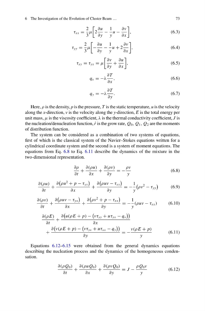
Here, ρ is the density, p is the pressure, T is the static temperature, u is the velocity
along the x-direction, v is the velocity along the y-direction, E is the total energy per
unit mass, μ is the viscosity coefficient, λ is the thermal conductivity coefficient, J is
the nucleation/denucleation function, ˙
r is the grow rate, Q 0 , Q 1 , Q 2 are the moments
of distribution function.
The system can be considered as a combination of two systems of equations,
first of which is the classical system of the Navier–Stokes equations written for a
cylindrical coordinate system and the second is a system of moment equations. The
equations from Eq. 6.8 to Eq. 6.11 describe the dynamics of the mixture in the
two-dimensional representation.
∂ρ
∂t
+
∂(ρu)
∂ x
+
∂(ρv)
∂ y
= −
ρv
y
(6.8)
∂(ρu)
∂t
+
∂
ρu
2
+ p − τ yy
∂ x
+
∂
ρuv − τ xy
∂ y
= −
1
y
ρv
2
− τ yy
(6.9)
∂(ρv)
∂t
+
∂
ρuv − τ yx
∂ x
+
∂
ρv
2
+ p − τ xx
∂ y
= −
1
y
(ρuv − τ xx )
(6.10)
∂(ρ E)
∂t
+
∂
u(ρ E + p) −
vτ yy + uτ yx − q x
∂ x
+
∂
v(ρ E + p) −
vτ yx + uτ xx − q y
∂ y
= −
v(ρ E + p)
y
(6.11)
Equations 6.12–6.15 were obtained from the general dynamics equations
describing the nucleation process and the dynamics of the homogeneous condensation.
∂(ρ Q 0 )
∂t
+
∂(ρu Q 0 )
∂ x
+
∂(ρvQ 0 )
∂ y
= J −
ρ Q 0 v
y
(6.12)
73
τ xx =
2
3
μ
2
∂u
∂ y
−
1
y
u −
∂v
∂ x
,
(6.3)
τ yy =
2
3
μ
−
∂u
∂ y
−
1
y
u + 2
∂v
∂ x
,
(6.4)
τ xy = τ yx = μ
∂v
∂ y
+
∂u
∂ x
,
(6.5)
q x = −λ
∂ T
∂ x
,
(6.6)
q y = −λ
∂ T
∂ y
.
(6.7)
Here, ρ is the density, p is the pressure, T is the static temperature, u is the velocity
along the x-direction, v is the velocity along the y-direction, E is the total energy per
unit mass, μ is the viscosity coefficient, λ is the thermal conductivity coefficient, J is
the nucleation/denucleation function, ˙
r is the grow rate, Q 0 , Q 1 , Q 2 are the moments
of distribution function.
The system can be considered as a combination of two systems of equations,
first of which is the classical system of the Navier–Stokes equations written for a
cylindrical coordinate system and the second is a system of moment equations. The
equations from Eq. 6.8 to Eq. 6.11 describe the dynamics of the mixture in the
two-dimensional representation.
∂ρ
∂t
+
∂(ρu)
∂ x
+
∂(ρv)
∂ y
= −
ρv
y
(6.8)
∂(ρu)
∂t
+
∂
ρu
2
+ p − τ yy
∂ x
+
∂
ρuv − τ xy
∂ y
= −
1
y
ρv
2
− τ yy
(6.9)
∂(ρv)
∂t
+
∂
ρuv − τ yx
∂ x
+
∂
ρv
2
+ p − τ xx
∂ y
= −
1
y
(ρuv − τ xx )
(6.10)
∂(ρ E)
∂t
+
∂
u(ρ E + p) −
vτ yy + uτ yx − q x
∂ x
+
∂
v(ρ E + p) −
vτ yx + uτ xx − q y
∂ y
= −
v(ρ E + p)
y
(6.11)
Equations 6.12–6.15 were obtained from the general dynamics equations
describing the nucleation process and the dynamics of the homogeneous condensation.
∂(ρ Q 0 )
∂t
+
∂(ρu Q 0 )
∂ x
+
∂(ρvQ 0 )
∂ y
= J −
ρ Q 0 v
y
(6.12)