

40
V. A. Gushchin et al.
class of problems is to numerically integrate the complete nonstationary hydrodynamic equations. The known methods for calculating viscous incompressible fluid
flows with a free surface do not allow obtaining highly accurate solutions near the
free surface and in areas of large gradients of hydrodynamic flow parameters. In this
respect, it is necessary to further develop methods of the numerical integration for
the complete hydrodynamic equations with a free surface.
For solving such problems, in [10], it was proposed a new differential scheme
based on CABARET method [3, 4]. The application of this approach for investigation
of flows with a free surface may be seen in [21]. In [12], it was proposed a new finitedifference scheme based on CABARET technique for solving the spot problem. The
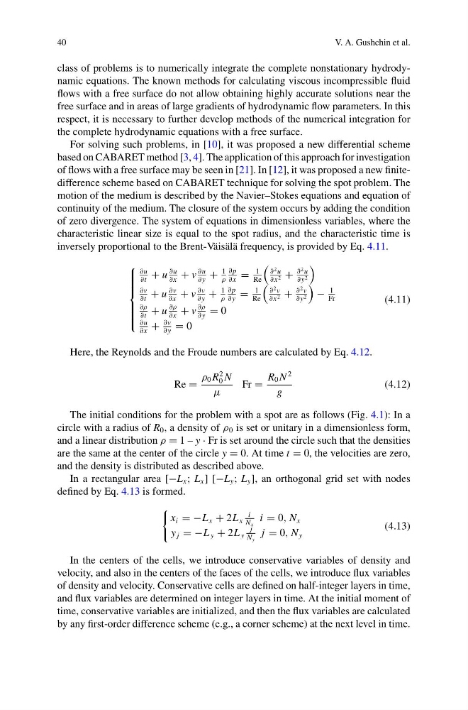
motion of the medium is described by the Navier–Stokes equations and equation of
continuity of the medium. The closure of the system occurs by adding the condition
of zero divergence. The system of equations in dimensionless variables, where the
characteristic linear size is equal to the spot radius, and the characteristic time is
inversely proportional to the Brent-Väisälä frequency, is provided by Eq. 4.11.
⎧
⎪ ⎪ ⎪ ⎪ ⎨
⎪ ⎪ ⎪ ⎪ ⎩
∂u
∂t
+ u
∂u
∂ x
+ v
∂u
∂ y
+
1
ρ
∂ p
∂ x
=
1
Re
∂
2 u
∂ x 2 +
∂
2 u
∂ y 2
∂v
∂t
+ u
∂v
∂ x
+ v
∂v
∂ y
+
1
ρ
∂ p
∂ y
=
1
Re
∂
2 v
∂ x 2 +
∂
2 v
∂ y 2
−
1
Fr
∂ρ
∂t
+ u
∂ρ
∂ x
+ v
∂ρ
∂ y
= 0
∂u
∂ x
+
∂v
∂ y
= 0
(4.11)
Here, the Reynolds and the Froude numbers are calculated by Eq. 4.12.
Re =
ρ 0 R
2
0 N
μ
Fr =
R 0 N
2
g
(4.12)
The initial conditions for the problem with a spot are as follows (Fig. 4.1): In a
circle with a radius of R 0 , a density of ρ 0 is set or unitary in a dimensionless form,
and a linear distribution ρ = 1 – y · Fr is set around the circle such that the densities
are the same at the center of the circle y = 0. At time t = 0, the velocities are zero,
and the density is distributed as described above.
In a rectangular area [−L x ; L x ] [−L y ; L y ], an orthogonal grid set with nodes
defined by Eq. 4.13 is formed.
x i = −L x + 2L x
i
N x
i = 0, N x
y j = −L y + 2L y
j
N y
j = 0, N y
(4.13)
In the centers of the cells, we introduce conservative variables of density and
velocity, and also in the centers of the faces of the cells, we introduce flux variables
of density and velocity. Conservative cells are defined on half-integer layers in time,
and flux variables are determined on integer layers in time. At the initial moment of
time, conservative variables are initialized, and then the flux variables are calculated
by any first-order difference scheme (e.g., a corner scheme) at the next level in time.
V. A. Gushchin et al.
class of problems is to numerically integrate the complete nonstationary hydrodynamic equations. The known methods for calculating viscous incompressible fluid
flows with a free surface do not allow obtaining highly accurate solutions near the
free surface and in areas of large gradients of hydrodynamic flow parameters. In this
respect, it is necessary to further develop methods of the numerical integration for
the complete hydrodynamic equations with a free surface.
For solving such problems, in [10], it was proposed a new differential scheme
based on CABARET method [3, 4]. The application of this approach for investigation
of flows with a free surface may be seen in [21]. In [12], it was proposed a new finitedifference scheme based on CABARET technique for solving the spot problem. The
motion of the medium is described by the Navier–Stokes equations and equation of
continuity of the medium. The closure of the system occurs by adding the condition
of zero divergence. The system of equations in dimensionless variables, where the
characteristic linear size is equal to the spot radius, and the characteristic time is
inversely proportional to the Brent-Väisälä frequency, is provided by Eq. 4.11.
⎧
⎪ ⎪ ⎪ ⎪ ⎨
⎪ ⎪ ⎪ ⎪ ⎩
∂u
∂t
+ u
∂u
∂ x
+ v
∂u
∂ y
+
1
ρ
∂ p
∂ x
=
1
Re
∂
2 u
∂ x 2 +
∂
2 u
∂ y 2
∂v
∂t
+ u
∂v
∂ x
+ v
∂v
∂ y
+
1
ρ
∂ p
∂ y
=
1
Re
∂
2 v
∂ x 2 +
∂
2 v
∂ y 2
−
1
Fr
∂ρ
∂t
+ u
∂ρ
∂ x
+ v
∂ρ
∂ y
= 0
∂u
∂ x
+
∂v
∂ y
= 0
(4.11)
Here, the Reynolds and the Froude numbers are calculated by Eq. 4.12.
Re =
ρ 0 R
2
0 N
μ
Fr =
R 0 N
2
g
(4.12)
The initial conditions for the problem with a spot are as follows (Fig. 4.1): In a
circle with a radius of R 0 , a density of ρ 0 is set or unitary in a dimensionless form,
and a linear distribution ρ = 1 – y · Fr is set around the circle such that the densities
are the same at the center of the circle y = 0. At time t = 0, the velocities are zero,
and the density is distributed as described above.
In a rectangular area [−L x ; L x ] [−L y ; L y ], an orthogonal grid set with nodes
defined by Eq. 4.13 is formed.
x i = −L x + 2L x
i
N x
i = 0, N x
y j = −L y + 2L y
j
N y
j = 0, N y
(4.13)
In the centers of the cells, we introduce conservative variables of density and
velocity, and also in the centers of the faces of the cells, we introduce flux variables
of density and velocity. Conservative cells are defined on half-integer layers in time,
and flux variables are determined on integer layers in time. At the initial moment of
time, conservative variables are initialized, and then the flux variables are calculated
by any first-order difference scheme (e.g., a corner scheme) at the next level in time.