

4 Mathematical Modeling of Wave Motions of Fluids
41
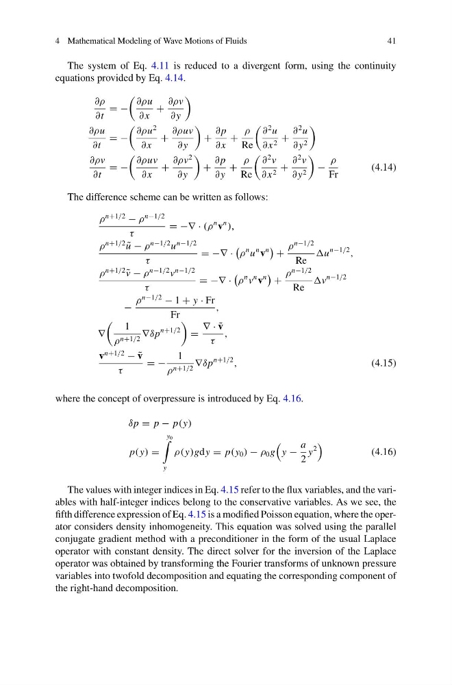
The system of Eq. 4.11 is reduced to a divergent form, using the continuity
equations provided by Eq. 4.14.
∂ρ
∂t
= −
∂ρu
∂ x
+
∂ρv
∂ y
∂ρu
∂t
= −
∂ρu
2
∂ x
+
∂ρuv
∂ y
+
∂ p
∂ x
+
ρ
Re
∂
2 u
∂ x 2 +
∂
2 u
∂ y 2
∂ρv
∂t
= −
∂ρuv
∂ x
+
∂ρv
2
∂ y
+
∂ p
∂ y
+
ρ
Re
∂
2 v
∂ x 2 +
∂
2 v
∂ y 2
−
ρ
Fr
(4.14)
The difference scheme can be written as follows:
ρ
n+1/2
− ρ
n−1/2
τ
= −∇ · (ρ
n v
n
),
ρ
n+1/2
˜
u − ρ
n−1/2 u
n−1/2
τ
= −∇ ·
ρ
n u
n v
n
+
ρ
n−1/2
Re
u
n−1/2
,
ρ
n+1/2
˜
v − ρ
n−1/2 v
n−1/2
τ
= −∇ ·
ρ
n v
n v
n
+
ρ
n−1/2
Re
v
n−1/2
−
ρ
n−1/2
− 1 + y · Fr
Fr
,
∇
1
ρ n+1/2 ∇δp
n+1/2
=
∇ · ˜
v
τ
,
v
n+1/2
− ˜
v
τ
= −
1
ρ n+1/2 ∇δp
n+1/2
,
(4.15)
where the concept of overpressure is introduced by Eq. 4.16.
δp = p − p(y)
p(y) =
y 0
y
ρ(y)gdy = p(y 0 ) − ρ 0 g
y −
a
2
y
2
(4.16)
The values with integer indices in Eq. 4.15 refer to the flux variables, and the variables with half-integer indices belong to the conservative variables. As we see, the
fifth difference expression of Eq. 4.15 is a modified Poisson equation, where the operator considers density inhomogeneity. This equation was solved using the parallel
conjugate gradient method with a preconditioner in the form of the usual Laplace
operator with constant density. The direct solver for the inversion of the Laplace
operator was obtained by transforming the Fourier transforms of unknown pressure
variables into twofold decomposition and equating the corresponding component of
the right-hand decomposition.
41
The system of Eq. 4.11 is reduced to a divergent form, using the continuity
equations provided by Eq. 4.14.
∂ρ
∂t
= −
∂ρu
∂ x
+
∂ρv
∂ y
∂ρu
∂t
= −
∂ρu
2
∂ x
+
∂ρuv
∂ y
+
∂ p
∂ x
+
ρ
Re
∂
2 u
∂ x 2 +
∂
2 u
∂ y 2
∂ρv
∂t
= −
∂ρuv
∂ x
+
∂ρv
2
∂ y
+
∂ p
∂ y
+
ρ
Re
∂
2 v
∂ x 2 +
∂
2 v
∂ y 2
−
ρ
Fr
(4.14)
The difference scheme can be written as follows:
ρ
n+1/2
− ρ
n−1/2
τ
= −∇ · (ρ
n v
n
),
ρ
n+1/2
˜
u − ρ
n−1/2 u
n−1/2
τ
= −∇ ·
ρ
n u
n v
n
+
ρ
n−1/2
Re
u
n−1/2
,
ρ
n+1/2
˜
v − ρ
n−1/2 v
n−1/2
τ
= −∇ ·
ρ
n v
n v
n
+
ρ
n−1/2
Re
v
n−1/2
−
ρ
n−1/2
− 1 + y · Fr
Fr
,
∇
1
ρ n+1/2 ∇δp
n+1/2
=
∇ · ˜
v
τ
,
v
n+1/2
− ˜
v
τ
= −
1
ρ n+1/2 ∇δp
n+1/2
,
(4.15)
where the concept of overpressure is introduced by Eq. 4.16.
δp = p − p(y)
p(y) =
y 0
y
ρ(y)gdy = p(y 0 ) − ρ 0 g
y −
a
2
y
2
(4.16)
The values with integer indices in Eq. 4.15 refer to the flux variables, and the variables with half-integer indices belong to the conservative variables. As we see, the
fifth difference expression of Eq. 4.15 is a modified Poisson equation, where the operator considers density inhomogeneity. This equation was solved using the parallel
conjugate gradient method with a preconditioner in the form of the usual Laplace
operator with constant density. The direct solver for the inversion of the Laplace
operator was obtained by transforming the Fourier transforms of unknown pressure
variables into twofold decomposition and equating the corresponding component of
the right-hand decomposition.