

21 Fractal Analysis and Programming of Elastic Systems …
315
A discrete-time system is denoted symbolically by
y[m] = f {u[m]},
(21.5)
where f denotes CCM characterizing the system.
In a box-counting method, it takes that a curve is given. Let a part of a curve
named sample is formed dynamically at a given time interval T.
Definition 5 Let N be the number of boxes calculated dynamically by function n: (δ
[m · T ], ε max ) → N, where δ [m · T ] is a curve sample calculated by Eq. 21.4, then
control signals u[m] is denoted by Eq. 21.6.
u[m] = u[m · T ] =
⎧
⎪ ⎨
⎪ ⎩
n left (δ[m · T ], ε max ) if m > m − 1
n right (δ[m · T ], ε max ) if m < m − 1
0
i fm ≤ 0
(21.6)
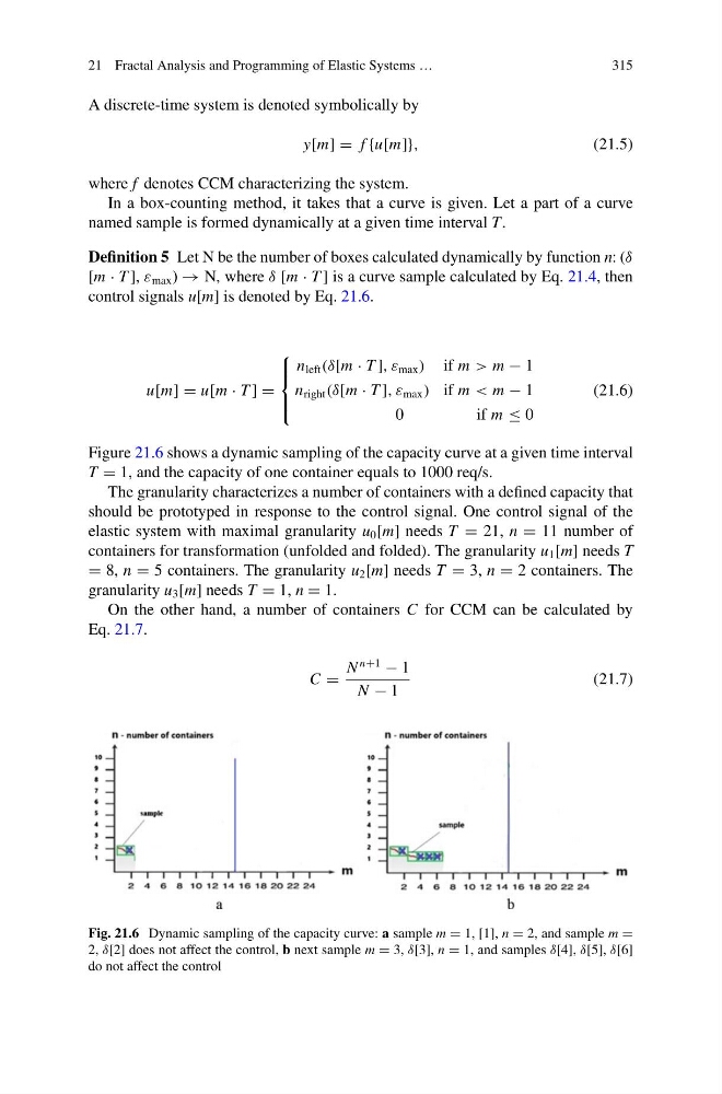
Figure 21.6 shows a dynamic sampling of the capacity curve at a given time interval
T = 1, and the capacity of one container equals to 1000 req/s.
The granularity characterizes a number of containers with a defined capacity that
should be prototyped in response to the control signal. One control signal of the
elastic system with maximal granularity u 0 [m] needs T = 21, n = 11 number of
containers for transformation (unfolded and folded). The granularity u 1 [m] needs T
= 8, n = 5 containers. The granularity u 2 [m] needs T = 3, n = 2 containers. The
granularity u 3 [m] needs T = 1, n = 1.
On the other hand, a number of containers C for CCM can be calculated by
Eq. 21.7.
C =
N
n+1
− 1
N − 1
(21.7)
Fig. 21.6 Dynamic sampling of the capacity curve: a sample m = 1, [1], n = 2, and sample m =
2, δ[2] does not affect the control, b next sample m = 3, δ[3], n = 1, and samples δ[4], δ[5], δ[6]
do not affect the control
315
A discrete-time system is denoted symbolically by
y[m] = f {u[m]},
(21.5)
where f denotes CCM characterizing the system.
In a box-counting method, it takes that a curve is given. Let a part of a curve
named sample is formed dynamically at a given time interval T.
Definition 5 Let N be the number of boxes calculated dynamically by function n: (δ
[m · T ], ε max ) → N, where δ [m · T ] is a curve sample calculated by Eq. 21.4, then
control signals u[m] is denoted by Eq. 21.6.
u[m] = u[m · T ] =
⎧
⎪ ⎨
⎪ ⎩
n left (δ[m · T ], ε max ) if m > m − 1
n right (δ[m · T ], ε max ) if m < m − 1
0
i fm ≤ 0
(21.6)
Figure 21.6 shows a dynamic sampling of the capacity curve at a given time interval
T = 1, and the capacity of one container equals to 1000 req/s.
The granularity characterizes a number of containers with a defined capacity that
should be prototyped in response to the control signal. One control signal of the
elastic system with maximal granularity u 0 [m] needs T = 21, n = 11 number of
containers for transformation (unfolded and folded). The granularity u 1 [m] needs T
= 8, n = 5 containers. The granularity u 2 [m] needs T = 3, n = 2 containers. The
granularity u 3 [m] needs T = 1, n = 1.
On the other hand, a number of containers C for CCM can be calculated by
Eq. 21.7.
C =
N
n+1
− 1
N − 1
(21.7)
Fig. 21.6 Dynamic sampling of the capacity curve: a sample m = 1, [1], n = 2, and sample m =
2, δ[2] does not affect the control, b next sample m = 3, δ[3], n = 1, and samples δ[4], δ[5], δ[6]
do not affect the control