

314
A. S. Semenov
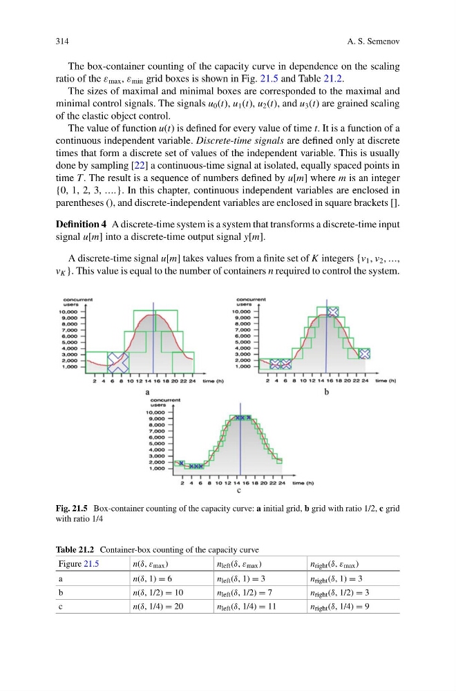
The box-container counting of the capacity curve in dependence on the scaling
ratio of the ε max , ε min grid boxes is shown in Fig. 21.5 and Table 21.2.
The sizes of maximal and minimal boxes are corresponded to the maximal and
minimal control signals. The signals u 0 (t), u 1 (t), u 2 (t), and u 3 (t) are grained scaling
of the elastic object control.
The value of function u(t) is defined for every value of time t. It is a function of a
continuous independent variable. Discrete-time signals are defined only at discrete
times that form a discrete set of values of the independent variable. This is usually
done by sampling [22] a continuous-time signal at isolated, equally spaced points in
time T. The result is a sequence of numbers defined by u[m] where m is an integer
{0, 1, 2, 3, ….}. In this chapter, continuous independent variables are enclosed in
parentheses (), and discrete-independent variables are enclosed in square brackets [].
Definition 4 A discrete-time system is a system that transforms a discrete-time input
signal u[m] into a discrete-time output signal y[m].
A discrete-time signal u[m] takes values from a finite set of K integers {v 1 , v 2 , …,
v K }. This value is equal to the number of containers n required to control the system.
Fig. 21.5 Box-container counting of the capacity curve: a initial grid, b grid with ratio 1/2, c grid
with ratio 1/4
Table 21.2 Container-box counting of the capacity curve
Figure 21.5
n(δ, ε max )
n left (δ, ε max )
n right (δ, ε max )
a
n(δ, 1) = 6
n left (δ, 1) = 3
n right (δ, 1) = 3
b
n(δ, 1/2) = 10
n left (δ, 1/2) = 7
n right (δ, 1/2) = 3
c
n(δ, 1/4) = 20
n left (δ, 1/4) = 11
n right (δ, 1/4) = 9
A. S. Semenov
The box-container counting of the capacity curve in dependence on the scaling
ratio of the ε max , ε min grid boxes is shown in Fig. 21.5 and Table 21.2.
The sizes of maximal and minimal boxes are corresponded to the maximal and
minimal control signals. The signals u 0 (t), u 1 (t), u 2 (t), and u 3 (t) are grained scaling
of the elastic object control.
The value of function u(t) is defined for every value of time t. It is a function of a
continuous independent variable. Discrete-time signals are defined only at discrete
times that form a discrete set of values of the independent variable. This is usually
done by sampling [22] a continuous-time signal at isolated, equally spaced points in
time T. The result is a sequence of numbers defined by u[m] where m is an integer
{0, 1, 2, 3, ….}. In this chapter, continuous independent variables are enclosed in
parentheses (), and discrete-independent variables are enclosed in square brackets [].
Definition 4 A discrete-time system is a system that transforms a discrete-time input
signal u[m] into a discrete-time output signal y[m].
A discrete-time signal u[m] takes values from a finite set of K integers {v 1 , v 2 , …,
v K }. This value is equal to the number of containers n required to control the system.
Fig. 21.5 Box-container counting of the capacity curve: a initial grid, b grid with ratio 1/2, c grid
with ratio 1/4
Table 21.2 Container-box counting of the capacity curve
Figure 21.5
n(δ, ε max )
n left (δ, ε max )
n right (δ, ε max )
a
n(δ, 1) = 6
n left (δ, 1) = 3
n right (δ, 1) = 3
b
n(δ, 1/2) = 10
n left (δ, 1/2) = 7
n right (δ, 1/2) = 3
c
n(δ, 1/4) = 20
n left (δ, 1/4) = 11
n right (δ, 1/4) = 9