

18 Incomplete Pairwise Comparisons Method for Estimating …
267
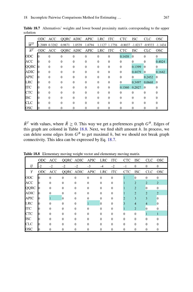
Table 18.7 Alternatives’ weights and lower bound proximity matrix corresponding to the upper
solution
ODC ACC QQRC ADIC APIC LRC ITC
CTC ISC
CLC OSC
1.2089 0.3282 0.9871 1.0539 1.0794 1.1127 1.1756 -0.8037 -1.0217 -0.9333 -1.1434
ODC ACC QQRC ADIC APIC LRC ITC
CTC ISC
CLC OSC
ODC 0
0
0
0
0
0
0
0.1438 0
0
0
ACC 0
0
0
0
0
0
0
0
0
0
0.4024
QQRC 0
0
0
0
0
0
0
0
0.1399 0
0
ADIC 0
0
0
0
0
0
0
0
0.4479 0
0.1642
APIC 0
0
0
0
0
0
0
0
0
0.2452 0
LRC 0
0
0
0
0
0
0
0
0.3497 0.0668 0
ITC
0
0
0
0
0
0
0
0.1560 0.2027 0
0
CTC 0
0
0
0
0
0
0
0
0
0
0
ISC
0
0
0
0
0
0
0
0
0
0
0
CLC 0
0
0
0
0
0
0
0
0
0
0
OSC 0
0
0
0
0
0
0
0
0
0
0
¯
R
T with values, where ¯
R ≥ 0. This way we get a preferences graph G
B . Edges of
this graph are colored in Table 18.8. Next, we find shift amount h. In process, we
can delete some edges from G
B to get maximal h, but we should not break graph
connectivity. This idea can be expressed by Eq. 18.7.
Table 18.8 Elementary moving weight vector and elementary moving matrix
ODC ACC QQRC ADIC APIC LRC ITC
CTC ISC CLC OSC
–2
– 2
– 2
– 2
– 3
– 4
– 2
– 1
0
0
0
ODC ACC QQRC ADIC APIC LRC ITC
CTC ISC CLC OSC
ODC 0
0
0
0
0
0
0
1
0
0
0
ACC 0
0
0
0
0
0
0
1
2
2
2
QQRC 0
0
0
0
0
0
0
1
2
0
0
ADIC 0
0
0
0
0
0
0
1
2
2
2
APIC 0
1
0
0
0
0
0
2
3
3
0
LRC
0
0
0
0
1
0
0
3
4
4
0
ITC
0
0
0
0
0
0
0
1
2
0
0
CTC
0
0
0
0
0
0
0
0
0
1
1
ISC
0
0
0
0
0
0
0
0
0
0
0
CLC
0
0
0
0
0
0
0
0
0
0
0
OSC
0
0
0
0
0
0
0
0
0
0
0
267
Table 18.7 Alternatives’ weights and lower bound proximity matrix corresponding to the upper
solution
ODC ACC QQRC ADIC APIC LRC ITC
CTC ISC
CLC OSC
1.2089 0.3282 0.9871 1.0539 1.0794 1.1127 1.1756 -0.8037 -1.0217 -0.9333 -1.1434
ODC ACC QQRC ADIC APIC LRC ITC
CTC ISC
CLC OSC
ODC 0
0
0
0
0
0
0
0.1438 0
0
0
ACC 0
0
0
0
0
0
0
0
0
0
0.4024
QQRC 0
0
0
0
0
0
0
0
0.1399 0
0
ADIC 0
0
0
0
0
0
0
0
0.4479 0
0.1642
APIC 0
0
0
0
0
0
0
0
0
0.2452 0
LRC 0
0
0
0
0
0
0
0
0.3497 0.0668 0
ITC
0
0
0
0
0
0
0
0.1560 0.2027 0
0
CTC 0
0
0
0
0
0
0
0
0
0
0
ISC
0
0
0
0
0
0
0
0
0
0
0
CLC 0
0
0
0
0
0
0
0
0
0
0
OSC 0
0
0
0
0
0
0
0
0
0
0
¯
R
T with values, where ¯
R ≥ 0. This way we get a preferences graph G
B . Edges of
this graph are colored in Table 18.8. Next, we find shift amount h. In process, we
can delete some edges from G
B to get maximal h, but we should not break graph
connectivity. This idea can be expressed by Eq. 18.7.
Table 18.8 Elementary moving weight vector and elementary moving matrix
ODC ACC QQRC ADIC APIC LRC ITC
CTC ISC CLC OSC
–2
– 2
– 2
– 2
– 3
– 4
– 2
– 1
0
0
0
ODC ACC QQRC ADIC APIC LRC ITC
CTC ISC CLC OSC
ODC 0
0
0
0
0
0
0
1
0
0
0
ACC 0
0
0
0
0
0
0
1
2
2
2
QQRC 0
0
0
0
0
0
0
1
2
0
0
ADIC 0
0
0
0
0
0
0
1
2
2
2
APIC 0
1
0
0
0
0
0
2
3
3
0
LRC
0
0
0
0
1
0
0
3
4
4
0
ITC
0
0
0
0
0
0
0
1
2
0
0
CTC
0
0
0
0
0
0
0
0
0
1
1
ISC
0
0
0
0
0
0
0
0
0
0
0
CLC
0
0
0
0
0
0
0
0
0
0
0
OSC
0
0
0
0
0
0
0
0
0
0
0