

266
N. M. Kuzmina and A. N. Ridley
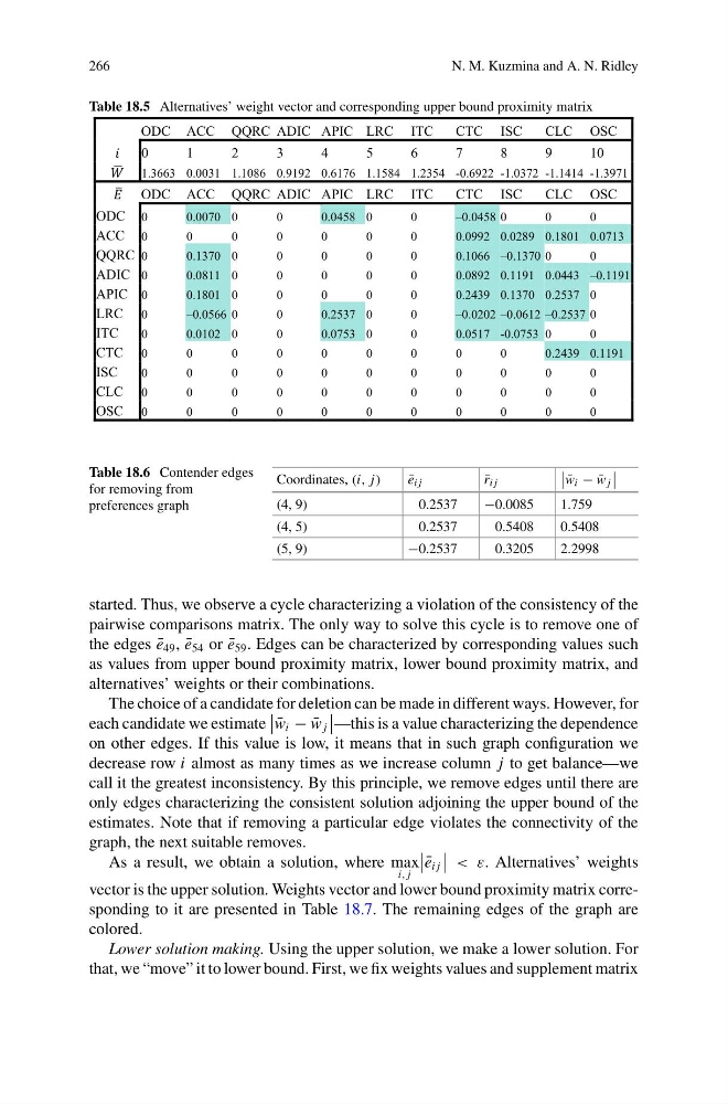
Table 18.5 Alternatives’ weight vector and corresponding upper bound proximity matrix
ODC ACC QQRC ADIC APIC LRC ITC
CTC ISC
CLC OSC
0
1
2
3
4
5
6
7
8
9
1 0
1.3663 0.0031 1.1086 0.9192 0.6176 1.1584 1.2354 -0.6922 -1.0372 -1.1414 -1.3971
ODC ACC QQRC ADIC APIC LRC ITC
CTC ISC
CLC OSC
ODC 0
0.0070 0
0
0.0458 0
0
–0.0458 0
0
0
ACC 0
0
0
0
0
0
0
0.0992 0.0289 0.1801 0.0713
QQRC 0
0.1370 0
0
0
0
0
0.1066 –0.1370 0
0
ADIC 0
0.0811 0
0
0
0
0
0.0892 0.1191 0.0443 –0.1191
APIC 0
0.1801 0
0
0
0
0
0.2439 0.1370 0.2537 0
LRC 0
–0.0566 0
0
0.2537 0
0
–0.0202 –0.0612 –0.2537 0
ITC
0
0.0102 0
0
0.0753 0
0
0.0517 -0.0753 0
0
CTC 0
0
0
0
0
0
0
0
0
0.2439 0.1191
ISC
0
0
0
0
0
0
0
0
0
0
0
CLC 0
0
0
0
0
0
0
0
0
0
0
OSC 0
0
0
0
0
0
0
0
0
0
0
Table 18.6 Contender edges
for removing from
preferences graph
Coordinates, (i, j)
¯
e i j
¯
r i j
¯
w i − ¯
w j
(4, 9)
0.2537
−0.0085
1.759
(4, 5)
0.2537
0.5408
0.5408
(5, 9)
−0.2537
0.3205
2.2998
started. Thus, we observe a cycle characterizing a violation of the consistency of the
pairwise comparisons matrix. The only way to solve this cycle is to remove one of
the edges ¯
e 49 , ¯
e 54 or ¯
e 59 . Edges can be characterized by corresponding values such
as values from upper bound proximity matrix, lower bound proximity matrix, and
alternatives’ weights or their combinations.
The choice of a candidate for deletion can be made in different ways. However, for
each candidate we estimate
¯
w i − ¯
w j
—this is a value characterizing the dependence
on other edges. If this value is low, it means that in such graph configuration we
decrease row i almost as many times as we increase column j to get balance—we
call it the greatest inconsistency. By this principle, we remove edges until there are
only edges characterizing the consistent solution adjoining the upper bound of the
estimates. Note that if removing a particular edge violates the connectivity of the
graph, the next suitable removes.
As a result, we obtain a solution, where max
i, j
¯
e i j
< ε. Alternatives’ weights
vector is the upper solution. Weights vector and lower bound proximity matrix corresponding to it are presented in Table 18.7. The remaining edges of the graph are
colored.
Lower solution making. Using the upper solution, we make a lower solution. For
that, we “move” it to lower bound. First, we fix weights values and supplement matrix
N. M. Kuzmina and A. N. Ridley
Table 18.5 Alternatives’ weight vector and corresponding upper bound proximity matrix
ODC ACC QQRC ADIC APIC LRC ITC
CTC ISC
CLC OSC
0
1
2
3
4
5
6
7
8
9
1 0
1.3663 0.0031 1.1086 0.9192 0.6176 1.1584 1.2354 -0.6922 -1.0372 -1.1414 -1.3971
ODC ACC QQRC ADIC APIC LRC ITC
CTC ISC
CLC OSC
ODC 0
0.0070 0
0
0.0458 0
0
–0.0458 0
0
0
ACC 0
0
0
0
0
0
0
0.0992 0.0289 0.1801 0.0713
QQRC 0
0.1370 0
0
0
0
0
0.1066 –0.1370 0
0
ADIC 0
0.0811 0
0
0
0
0
0.0892 0.1191 0.0443 –0.1191
APIC 0
0.1801 0
0
0
0
0
0.2439 0.1370 0.2537 0
LRC 0
–0.0566 0
0
0.2537 0
0
–0.0202 –0.0612 –0.2537 0
ITC
0
0.0102 0
0
0.0753 0
0
0.0517 -0.0753 0
0
CTC 0
0
0
0
0
0
0
0
0
0.2439 0.1191
ISC
0
0
0
0
0
0
0
0
0
0
0
CLC 0
0
0
0
0
0
0
0
0
0
0
OSC 0
0
0
0
0
0
0
0
0
0
0
Table 18.6 Contender edges
for removing from
preferences graph
Coordinates, (i, j)
¯
e i j
¯
r i j
¯
w i − ¯
w j
(4, 9)
0.2537
−0.0085
1.759
(4, 5)
0.2537
0.5408
0.5408
(5, 9)
−0.2537
0.3205
2.2998
started. Thus, we observe a cycle characterizing a violation of the consistency of the
pairwise comparisons matrix. The only way to solve this cycle is to remove one of
the edges ¯
e 49 , ¯
e 54 or ¯
e 59 . Edges can be characterized by corresponding values such
as values from upper bound proximity matrix, lower bound proximity matrix, and
alternatives’ weights or their combinations.
The choice of a candidate for deletion can be made in different ways. However, for
each candidate we estimate
¯
w i − ¯
w j
—this is a value characterizing the dependence
on other edges. If this value is low, it means that in such graph configuration we
decrease row i almost as many times as we increase column j to get balance—we
call it the greatest inconsistency. By this principle, we remove edges until there are
only edges characterizing the consistent solution adjoining the upper bound of the
estimates. Note that if removing a particular edge violates the connectivity of the
graph, the next suitable removes.
As a result, we obtain a solution, where max
i, j
¯
e i j
< ε. Alternatives’ weights
vector is the upper solution. Weights vector and lower bound proximity matrix corresponding to it are presented in Table 18.7. The remaining edges of the graph are
colored.
Lower solution making. Using the upper solution, we make a lower solution. For
that, we “move” it to lower bound. First, we fix weights values and supplement matrix