

18 Incomplete Pairwise Comparisons Method for Estimating …
265
better orientation. Finally, we got upper and lower bounds of the expert’s preferences.
Their presence or absence can be defined with graph G, whose adjacency matrix is
represented in Table 18.4.
18.3.4 Weights Calculating
Preparatory stage. At this stage, we go to the logarithmic scale. All matrices, vectors,
and constants except matrix of preferences graph are calculating in logarithmic scale
to increase accuracy and make it easier. Next, we denote logarithmic equivalents of
linear quantities with the dash above. Logarithmic bounds are calculated by Eq. 18.5.
¯
b i j = ln b i j ¯
t i j = ln t i j
(18.5)
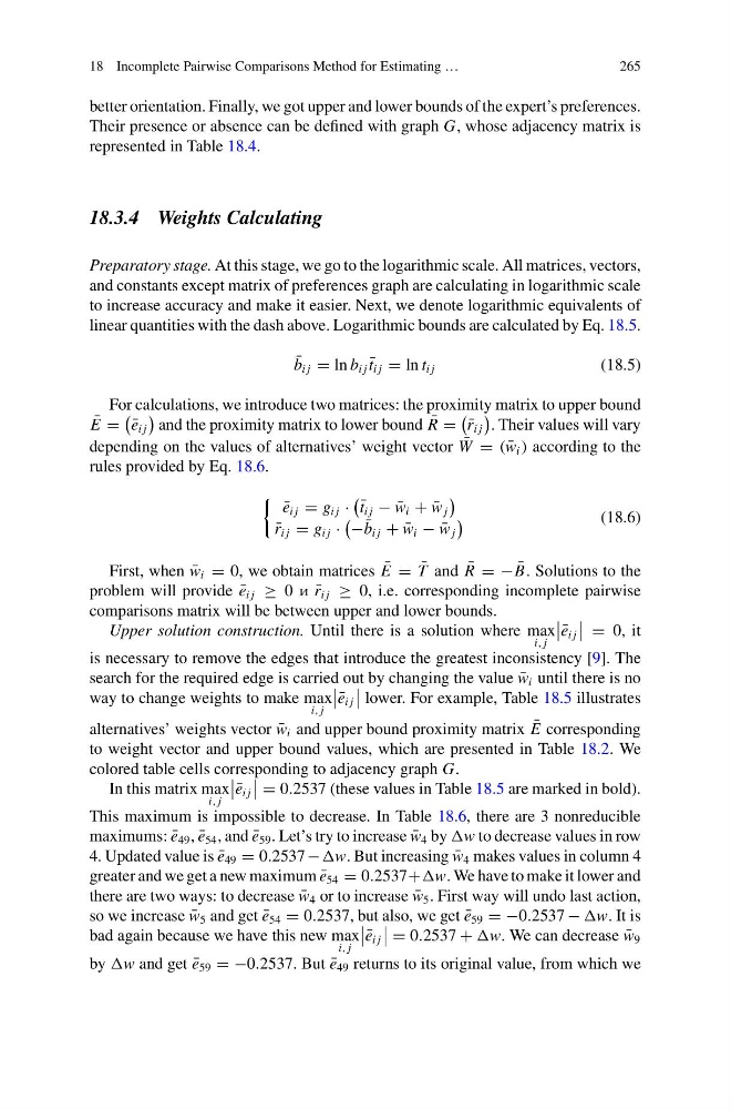
For calculations, we introduce two matrices: the proximity matrix to upper bound
¯
E =
¯
e i j
and the proximity matrix to lower bound ¯
R =
¯
r i j
. Their values will vary
depending on the values of alternatives’ weight vector ¯
W = ( ¯
w i ) according to the
rules provided by Eq. 18.6.
¯
e i j = g i j ·
¯
t i j − ¯
w i + ¯
w j
¯
r i j = g i j ·
− ¯
b i j + ¯
w i − ¯
w j
(18.6)
First, when ¯
w i = 0, we obtain matrices ¯
E = ¯
T and ¯
R = − ¯
B. Solutions to the
problem will provide ¯
e i j ≥ 0 i ¯
r i j ≥ 0, i.e. corresponding incomplete pairwise
comparisons matrix will be between upper and lower bounds.
Upper solution construction. Until there is a solution where max
i, j
¯
e i j
= 0, it
is necessary to remove the edges that introduce the greatest inconsistency [9]. The
search for the required edge is carried out by changing the value ¯
w i until there is no
way to change weights to make max
i, j
¯
e i j
lower. For example, Table 18.5 illustrates
alternatives’ weights vector ¯
w i and upper bound proximity matrix ¯
E corresponding
to weight vector and upper bound values, which are presented in Table 18.2. We
colored table cells corresponding to adjacency graph G.
In this matrix max
i, j
¯
e i j
= 0.2537 (these values in Table 18.5 are marked in bold).
This maximum is impossible to decrease. In Table 18.6, there are 3 nonreducible
maximums: ¯
e 49 , ¯
e 54 , and ¯
e 59 . Let’s try to increase ¯
w 4 by w to decrease values in row
4. Updated value is ¯
e 49 = 0.2537 − w. But increasing ¯
w 4 makes values in column 4
greater and we get a new maximum ¯
e 54 = 0.2537+w. We have to make it lower and
there are two ways: to decrease ¯
w 4 or to increase ¯
w 5 . First way will undo last action,
so we increase ¯
w 5 and get ¯
e 54 = 0.2537, but also, we get ¯
e 59 = −0.2537 − w. It is
bad again because we have this new max
i, j
¯
e i j
= 0.2537 + w. We can decrease ¯
w 9
by w and get ¯
e 59 = −0.2537. But ¯
e 49 returns to its original value, from which we
265
better orientation. Finally, we got upper and lower bounds of the expert’s preferences.
Their presence or absence can be defined with graph G, whose adjacency matrix is
represented in Table 18.4.
18.3.4 Weights Calculating
Preparatory stage. At this stage, we go to the logarithmic scale. All matrices, vectors,
and constants except matrix of preferences graph are calculating in logarithmic scale
to increase accuracy and make it easier. Next, we denote logarithmic equivalents of
linear quantities with the dash above. Logarithmic bounds are calculated by Eq. 18.5.
¯
b i j = ln b i j ¯
t i j = ln t i j
(18.5)
For calculations, we introduce two matrices: the proximity matrix to upper bound
¯
E =
¯
e i j
and the proximity matrix to lower bound ¯
R =
¯
r i j
. Their values will vary
depending on the values of alternatives’ weight vector ¯
W = ( ¯
w i ) according to the
rules provided by Eq. 18.6.
¯
e i j = g i j ·
¯
t i j − ¯
w i + ¯
w j
¯
r i j = g i j ·
− ¯
b i j + ¯
w i − ¯
w j
(18.6)
First, when ¯
w i = 0, we obtain matrices ¯
E = ¯
T and ¯
R = − ¯
B. Solutions to the
problem will provide ¯
e i j ≥ 0 i ¯
r i j ≥ 0, i.e. corresponding incomplete pairwise
comparisons matrix will be between upper and lower bounds.
Upper solution construction. Until there is a solution where max
i, j
¯
e i j
= 0, it
is necessary to remove the edges that introduce the greatest inconsistency [9]. The
search for the required edge is carried out by changing the value ¯
w i until there is no
way to change weights to make max
i, j
¯
e i j
lower. For example, Table 18.5 illustrates
alternatives’ weights vector ¯
w i and upper bound proximity matrix ¯
E corresponding
to weight vector and upper bound values, which are presented in Table 18.2. We
colored table cells corresponding to adjacency graph G.
In this matrix max
i, j
¯
e i j
= 0.2537 (these values in Table 18.5 are marked in bold).
This maximum is impossible to decrease. In Table 18.6, there are 3 nonreducible
maximums: ¯
e 49 , ¯
e 54 , and ¯
e 59 . Let’s try to increase ¯
w 4 by w to decrease values in row
4. Updated value is ¯
e 49 = 0.2537 − w. But increasing ¯
w 4 makes values in column 4
greater and we get a new maximum ¯
e 54 = 0.2537+w. We have to make it lower and
there are two ways: to decrease ¯
w 4 or to increase ¯
w 5 . First way will undo last action,
so we increase ¯
w 5 and get ¯
e 54 = 0.2537, but also, we get ¯
e 59 = −0.2537 − w. It is
bad again because we have this new max
i, j
¯
e i j
= 0.2537 + w. We can decrease ¯
w 9
by w and get ¯
e 59 = −0.2537. But ¯
e 49 returns to its original value, from which we