

240
A. V. Panteleev and M. M. S. Karane
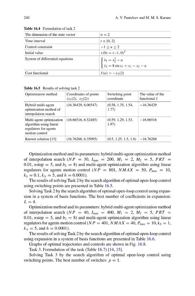
Table 16.4 Formulation of task 2
The dimension of the state vector
n = 2
Time interval
t ∈ [0, 2]
Control constraint
−1 ≤ u ≤ 2
Initial value
x(0) = (−1, 0) T
System of differential equations
˙
x 1 = x
2
2 + u
˙
x 2 = 8 sin x 1 + x 1 − x 2 − u
Cost functional
I (u) = −x 2 (2)
Table 16.5 Results of solving task 2
Optimization method
Coordinates of points
(x 1 (2), x 2 (2))
Switching point
coordinate
The value of the
functional I
Hybrid multi-agent
optimization method of
interpolation search
(16.36429, 6.06547)
(0.58, 1.35, 1.54,
1.77)
−16.36429
Multi-agent optimization
algorithm using linear
regulators for agents
motion control
(16.66516, 6.52485)
(0.59, 1.29, 1.53,
1.97)
−16.66516
Known solution [15]
(16.76268, 6.35095)
(0.5, 1.25, 1.5, 1.8) −16.76268
Optimization method and its parameters: hybrid multi-agent optimization method
of interpolation search (N P = 30, I max = 200, M 1 = 2, M 2 = 5, P RT =
0.01, nstep = 5, and b 2 = 8) and multi-agent optimization algorithm using linear
regulators for agents motion control (N P = 801, N M AX = 50, P max = 10,
k S = 0.1, k = 5, and h = 0.0001).
The results of solving Task 2 by the search algorithm of optimal open-loop control
using switching points are presented in Table 16.5.
Solving Task 2 by the search algorithm of optimal open-loop control using expansion in a system of basis functions. The best number of coefficients in expansion:
L = 4.
Optimization method and its parameters: hybrid multi-agent optimization method
of interpolation search (N P = 40, I max = 400, M 1 = 2, M 2 = 5, P RT =
0.01, nstep = 5, and b 2 = 8) and multi-agent optimization algorithm using linear
regulators for agents motion control (N P = 401, N M AX = 40, P max = 10, k S = 1,
k = 5, and h = 0.0001).
The results of solving Task 2 by the search algorithm of optimal open-loop control
using expansion in a system of basis functions are presented in Table 16.6.
Graphs of optimal trajectories and controls are shown in Fig. 16.8.
Task 3. Formulation of the task (Table 16.7) [14, 15].
Solving Task 3 by the search algorithm of optimal open-loop control using
switching points. The best number of switches: p = 1.
A. V. Panteleev and M. M. S. Karane
Table 16.4 Formulation of task 2
The dimension of the state vector
n = 2
Time interval
t ∈ [0, 2]
Control constraint
−1 ≤ u ≤ 2
Initial value
x(0) = (−1, 0) T
System of differential equations
˙
x 1 = x
2
2 + u
˙
x 2 = 8 sin x 1 + x 1 − x 2 − u
Cost functional
I (u) = −x 2 (2)
Table 16.5 Results of solving task 2
Optimization method
Coordinates of points
(x 1 (2), x 2 (2))
Switching point
coordinate
The value of the
functional I
Hybrid multi-agent
optimization method of
interpolation search
(16.36429, 6.06547)
(0.58, 1.35, 1.54,
1.77)
−16.36429
Multi-agent optimization
algorithm using linear
regulators for agents
motion control
(16.66516, 6.52485)
(0.59, 1.29, 1.53,
1.97)
−16.66516
Known solution [15]
(16.76268, 6.35095)
(0.5, 1.25, 1.5, 1.8) −16.76268
Optimization method and its parameters: hybrid multi-agent optimization method
of interpolation search (N P = 30, I max = 200, M 1 = 2, M 2 = 5, P RT =
0.01, nstep = 5, and b 2 = 8) and multi-agent optimization algorithm using linear
regulators for agents motion control (N P = 801, N M AX = 50, P max = 10,
k S = 0.1, k = 5, and h = 0.0001).
The results of solving Task 2 by the search algorithm of optimal open-loop control
using switching points are presented in Table 16.5.
Solving Task 2 by the search algorithm of optimal open-loop control using expansion in a system of basis functions. The best number of coefficients in expansion:
L = 4.
Optimization method and its parameters: hybrid multi-agent optimization method
of interpolation search (N P = 40, I max = 400, M 1 = 2, M 2 = 5, P RT =
0.01, nstep = 5, and b 2 = 8) and multi-agent optimization algorithm using linear
regulators for agents motion control (N P = 401, N M AX = 40, P max = 10, k S = 1,
k = 5, and h = 0.0001).
The results of solving Task 2 by the search algorithm of optimal open-loop control
using expansion in a system of basis functions are presented in Table 16.6.
Graphs of optimal trajectories and controls are shown in Fig. 16.8.
Task 3. Formulation of the task (Table 16.7) [14, 15].
Solving Task 3 by the search algorithm of optimal open-loop control using
switching points. The best number of switches: p = 1.