

16 Application of Multi-agent Optimization Methods …
241
Table 16.6 Results of solving task 2
Optimization method
Coordinates of points
(x 1 (2), x 2 (2))
Coefficients in
expansion c i
The value of the
functional I
Hybrid multi-agent
optimization method of
interpolation search
(13.01829, 4.44509)
−0.23, 1.73, 1.78,
1.81
−13,01,829
Multi-agent optimization
algorithm using linear
regulators for agents
motion control
(12.36497, 4.16002)
−0.28, 1.61, 1.79,
1.92
−12,36,497
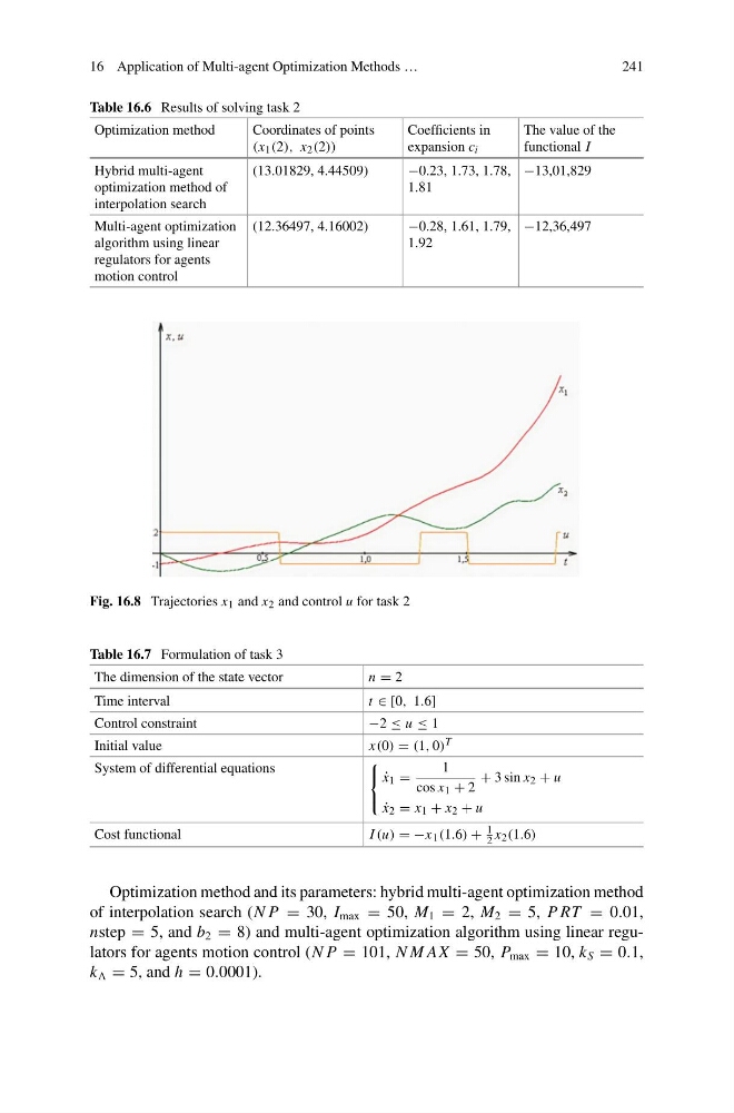
Fig. 16.8 Trajectories x 1 and x 2 and control u for task 2
Table 16.7 Formulation of task 3
The dimension of the state vector
n = 2
Time interval
t ∈ [0, 1.6]
Control constraint
−2 ≤ u ≤ 1
Initial value
x(0) = (1, 0) T
System of differential equations
⎧
⎨
⎩
˙
x 1 =
1
cos x 1 + 2
+ 3 sin x 2 + u
˙
x 2 = x 1 + x 2 + u
Cost functional
I (u) = −x 1 (1.6) +
1
2 x 2 (1.6)
Optimization method and its parameters: hybrid multi-agent optimization method
of interpolation search (N P = 30, I max = 50, M 1 = 2, M 2 = 5, P RT = 0.01,
nstep = 5, and b 2 = 8) and multi-agent optimization algorithm using linear regulators for agents motion control (N P = 101, N M AX = 50, P max = 10, k S = 0.1,
k = 5, and h = 0.0001).
241
Table 16.6 Results of solving task 2
Optimization method
Coordinates of points
(x 1 (2), x 2 (2))
Coefficients in
expansion c i
The value of the
functional I
Hybrid multi-agent
optimization method of
interpolation search
(13.01829, 4.44509)
−0.23, 1.73, 1.78,
1.81
−13,01,829
Multi-agent optimization
algorithm using linear
regulators for agents
motion control
(12.36497, 4.16002)
−0.28, 1.61, 1.79,
1.92
−12,36,497
Fig. 16.8 Trajectories x 1 and x 2 and control u for task 2
Table 16.7 Formulation of task 3
The dimension of the state vector
n = 2
Time interval
t ∈ [0, 1.6]
Control constraint
−2 ≤ u ≤ 1
Initial value
x(0) = (1, 0) T
System of differential equations
⎧
⎨
⎩
˙
x 1 =
1
cos x 1 + 2
+ 3 sin x 2 + u
˙
x 2 = x 1 + x 2 + u
Cost functional
I (u) = −x 1 (1.6) +
1
2 x 2 (1.6)
Optimization method and its parameters: hybrid multi-agent optimization method
of interpolation search (N P = 30, I max = 50, M 1 = 2, M 2 = 5, P RT = 0.01,
nstep = 5, and b 2 = 8) and multi-agent optimization algorithm using linear regulators for agents motion control (N P = 101, N M AX = 50, P max = 10, k S = 0.1,
k = 5, and h = 0.0001).