

120
A. G. Aksenov
a
b
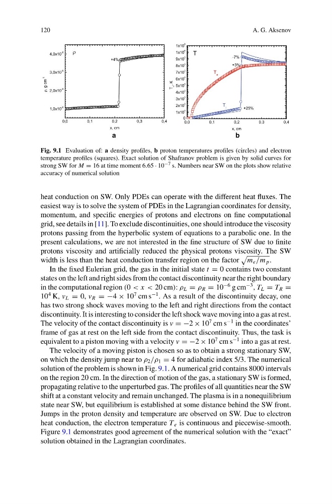
Fig. 9.1 Evaluation of: a density profiles, b proton temperatures profiles (circles) and electron
temperature profiles (squares). Exact solution of Shafranov problem is given by solid curves for
strong SW for M = 16 at time moment 6.65 · 10 −7 s. Numbers near SW on the plots show relative
accuracy of numerical solution
heat conduction on SW. Only PDEs can operate with the different heat fluxes. The
easiest way is to solve the system of PDEs in the Lagrangian coordinates for density,
momentum, and specific energies of protons and electrons on fine computational
grid, see details in [11]. To exclude discontinuities, one should introduce the viscosity
protons passing from the hyperbolic system of equations to a parabolic one. In the
present calculations, we are not interested in the fine structure of SW due to finite
protons viscosity and artificially reduced the physical protons viscosity. The SW
width is less than the heat conduction transfer region on the factor
m e /m p .
In the fixed Eulerian grid, the gas in the initial state t = 0 contains two constant
states on the left and right sides from the contact discontinuity near the right boundary
in the computational region (0 < x < 20 cm): ρ L = ρ R = 10
−6 g cm
−3 , T L = T R =
10
4 K, v L = 0, v R = −4 × 10
7 cm s
−1 . As a result of the discontinuity decay, one
has two strong shock waves moving to the left and right directions from the contact
discontinuity. It is interesting to consider the left shock wave moving into a gas at rest.
The velocity of the contact discontinuity is v = −2 × 10
7 cm s
−1 in the coordinates’
frame of gas at rest on the left side from the contact discontinuity. Thus, the task is
equivalent to a piston moving with a velocity v = −2 × 10
7 cm s
−1 into a gas at rest.
The velocity of a moving piston is chosen so as to obtain a strong stationary SW,
on which the density jump near to ρ 2 /ρ 1 = 4 for adiabatic index 5/3. The numerical
solution of the problem is shown in Fig. 9.1. A numerical grid contains 8000 intervals
on the region 20 cm. In the direction of motion of the gas, a stationary SW is formed,
propagating relative to the unperturbed gas. The profiles of all quantities near the SW
shift at a constant velocity and remain unchanged. The plasma is in a nonequilibrium
state near SW, but equilibrium is established at some distance behind the SW front.
Jumps in the proton density and temperature are observed on SW. Due to electron
heat conduction, the electron temperature T e is continuous and piecewise-smooth.
Figure 9.1 demonstrates good agreement of the numerical solution with the “exact”
solution obtained in the Lagrangian coordinates.
A. G. Aksenov
a
b
Fig. 9.1 Evaluation of: a density profiles, b proton temperatures profiles (circles) and electron
temperature profiles (squares). Exact solution of Shafranov problem is given by solid curves for
strong SW for M = 16 at time moment 6.65 · 10 −7 s. Numbers near SW on the plots show relative
accuracy of numerical solution
heat conduction on SW. Only PDEs can operate with the different heat fluxes. The
easiest way is to solve the system of PDEs in the Lagrangian coordinates for density,
momentum, and specific energies of protons and electrons on fine computational
grid, see details in [11]. To exclude discontinuities, one should introduce the viscosity
protons passing from the hyperbolic system of equations to a parabolic one. In the
present calculations, we are not interested in the fine structure of SW due to finite
protons viscosity and artificially reduced the physical protons viscosity. The SW
width is less than the heat conduction transfer region on the factor
m e /m p .
In the fixed Eulerian grid, the gas in the initial state t = 0 contains two constant
states on the left and right sides from the contact discontinuity near the right boundary
in the computational region (0 < x < 20 cm): ρ L = ρ R = 10
−6 g cm
−3 , T L = T R =
10
4 K, v L = 0, v R = −4 × 10
7 cm s
−1 . As a result of the discontinuity decay, one
has two strong shock waves moving to the left and right directions from the contact
discontinuity. It is interesting to consider the left shock wave moving into a gas at rest.
The velocity of the contact discontinuity is v = −2 × 10
7 cm s
−1 in the coordinates’
frame of gas at rest on the left side from the contact discontinuity. Thus, the task is
equivalent to a piston moving with a velocity v = −2 × 10
7 cm s
−1 into a gas at rest.
The velocity of a moving piston is chosen so as to obtain a strong stationary SW,
on which the density jump near to ρ 2 /ρ 1 = 4 for adiabatic index 5/3. The numerical
solution of the problem is shown in Fig. 9.1. A numerical grid contains 8000 intervals
on the region 20 cm. In the direction of motion of the gas, a stationary SW is formed,
propagating relative to the unperturbed gas. The profiles of all quantities near the SW
shift at a constant velocity and remain unchanged. The plasma is in a nonequilibrium
state near SW, but equilibrium is established at some distance behind the SW front.
Jumps in the proton density and temperature are observed on SW. Due to electron
heat conduction, the electron temperature T e is continuous and piecewise-smooth.
Figure 9.1 demonstrates good agreement of the numerical solution with the “exact”
solution obtained in the Lagrangian coordinates.