

208
6 Steam Turbines
Even with a symmetrical blade form, as represented in Fig. 6.9, axial velocity
decreases from inlet to outlet ( w 1a > w 2a ) due to losses. Further, the fluid density
decreases somewhat due to heating at constant pressure by losses ( ρ 1 > ρ 2 ). Both effects cause the need of a diverging meridional shape of the blade (Fig. 6.10, right).
At the periphery and the hub, the section area increase causes flow curvature in
the meridional plane. The associated pressure decrease on the concave side of the
streamsurfaces adds load to the boundary layer at the suction side trailing edge.
This implies that for a symmetrical blade, the divergence of the meridional section
is close to the possible maximum. In practice, β 2 = − β 1 , i.e. a symmetrical blade, is
mostly opted for. At most only a few degrees of deviation from symmetry are possible. Henceforth we take β 2 = − β 1 for the further analysis.
6.4.5 Loss Representation
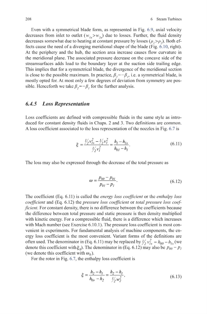
Loss coefficients are defined with compressible fluids in the same style as introduced for constant density fluids in Chaps. 2 and 3. Two definitions are common.
A loss coefficient associated to the loss representation of the nozzles in Fig. 6.7 is
(6.11)
The loss may also be expressed through the decrease of the total pressure as
(6.12)
The coefficient (Eq. 6.11) is called the energy loss coefficient or the enthalpy loss
coefficient and (Eq. 6.12) the pressure loss coefficient or total pressure loss coefficient. For constant density, there is no difference between the coefficients because
the difference between total pressure and static pressure is then density multiplied
with kinetic energy. For a compressible fluid, there is a difference which increases
with Mach number (see Exercise 6.10.1). The pressure loss coefficient is most convenient in experiments. For fundamental analysis of machine components, the energy loss coefficient is the most convenient. Variant forms of the definitions are
often used. The denominator in (Eq. 6.11) may be replaced by 1 2 1
2
00
1
v
h
h
s
s
=
− (we
denote this coefficient with 0
x ). The denominator in (Eq. 6.12) may also be p
p
00
1
−
(we denote this coefficient with 0
w ).
For the rotor in Fig. 6.7, the enthalpy loss coefficient is
(6.13)
2
2
1
1
1s
1
1
1s
2
2
2
1
01
1
1
2
v
v
h h .
h
h
v
x
−
−
=
=
−
.
00
01
01
1
p
p
p
p
w
−
=
−
2
1
2
1
2
1
0r
2
2
2
h h
h h ,
h
h
w
x
−
−
=
=
−
6 Steam Turbines
Even with a symmetrical blade form, as represented in Fig. 6.9, axial velocity
decreases from inlet to outlet ( w 1a > w 2a ) due to losses. Further, the fluid density
decreases somewhat due to heating at constant pressure by losses ( ρ 1 > ρ 2 ). Both effects cause the need of a diverging meridional shape of the blade (Fig. 6.10, right).
At the periphery and the hub, the section area increase causes flow curvature in
the meridional plane. The associated pressure decrease on the concave side of the
streamsurfaces adds load to the boundary layer at the suction side trailing edge.
This implies that for a symmetrical blade, the divergence of the meridional section
is close to the possible maximum. In practice, β 2 = − β 1 , i.e. a symmetrical blade, is
mostly opted for. At most only a few degrees of deviation from symmetry are possible. Henceforth we take β 2 = − β 1 for the further analysis.
6.4.5 Loss Representation
Loss coefficients are defined with compressible fluids in the same style as introduced for constant density fluids in Chaps. 2 and 3. Two definitions are common.
A loss coefficient associated to the loss representation of the nozzles in Fig. 6.7 is
(6.11)
The loss may also be expressed through the decrease of the total pressure as
(6.12)
The coefficient (Eq. 6.11) is called the energy loss coefficient or the enthalpy loss
coefficient and (Eq. 6.12) the pressure loss coefficient or total pressure loss coefficient. For constant density, there is no difference between the coefficients because
the difference between total pressure and static pressure is then density multiplied
with kinetic energy. For a compressible fluid, there is a difference which increases
with Mach number (see Exercise 6.10.1). The pressure loss coefficient is most convenient in experiments. For fundamental analysis of machine components, the energy loss coefficient is the most convenient. Variant forms of the definitions are
often used. The denominator in (Eq. 6.11) may be replaced by 1 2 1
2
00
1
v
h
h
s
s
=
− (we
denote this coefficient with 0
x ). The denominator in (Eq. 6.12) may also be p
p
00
1
−
(we denote this coefficient with 0
w ).
For the rotor in Fig. 6.7, the enthalpy loss coefficient is
(6.13)
2
2
1
1
1s
1
1
1s
2
2
2
1
01
1
1
2
v
v
h h .
h
h
v
x
−
−
=
=
−
.
00
01
01
1
p
p
p
p
w
−
=
−
2
1
2
1
2
1
0r
2
2
2
h h
h h ,
h
h
w
x
−
−
=
=
−