

199
6.3 The Steam Cycle
in opposite senses. The flow is centrifugal through the machine. This is inadequate
for a turbine, as it should be flowed through centripetally, but a centripetal design
is impossible, as the very high density drop with expansion requires an outlet area
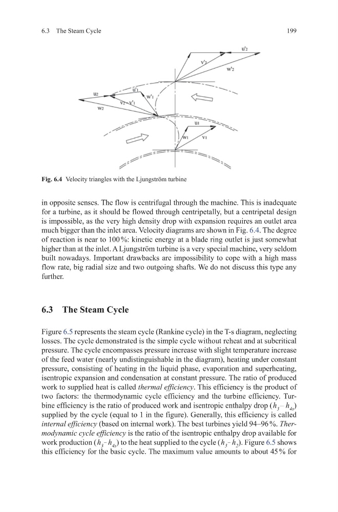
much bigger than the inlet area. Velocity diagrams are shown in Fig. 6.4. The degree
of reaction is near to 100 %: kinetic energy at a blade ring outlet is just somewhat
higher than at the inlet. A Ljungström turbine is a very special machine, very seldom
built nowadays. Important drawbacks are impossibility to cope with a high mass
flow rate, big radial size and two outgoing shafts. We do not discuss this type any
further.
6.3 The Steam Cycle
Figure 6.5 represents the steam cycle (Rankine cycle) in the T-s diagram, neglecting
losses. The cycle demonstrated is the simple cycle without reheat and at subcritical
pressure. The cycle encompasses pressure increase with slight temperature increase
of the feed water (nearly undistinguishable in the diagram), heating under constant
pressure, consisting of heating in the liquid phase, evaporation and superheating,
isentropic expansion and condensation at constant pressure. The ratio of produced
work to supplied heat is called thermal efficiency. This efficiency is the product of
two factors: the thermodynamic cycle efficiency and the turbine efficiency. Turbine efficiency is the ratio of produced work and isentropic enthalpy drop ( h 3 – h 4s )
supplied by the cycle (equal to 1 in the figure). Generally, this efficiency is called
internal efficiency (based on internal work). The best turbines yield 94–96 %. Thermodynamic cycle efficiency is the ratio of the isentropic enthalpy drop available for
work production ( h 3
– h 4s ) to the heat supplied to the cycle ( h 3
– h 2 ). Figure 6.5 shows
this efficiency for the basic cycle. The maximum value amounts to about 45 % for
Fig. 6.4 Velocity triangles with the Ljungström turbine
6.3 The Steam Cycle
in opposite senses. The flow is centrifugal through the machine. This is inadequate
for a turbine, as it should be flowed through centripetally, but a centripetal design
is impossible, as the very high density drop with expansion requires an outlet area
much bigger than the inlet area. Velocity diagrams are shown in Fig. 6.4. The degree
of reaction is near to 100 %: kinetic energy at a blade ring outlet is just somewhat
higher than at the inlet. A Ljungström turbine is a very special machine, very seldom
built nowadays. Important drawbacks are impossibility to cope with a high mass
flow rate, big radial size and two outgoing shafts. We do not discuss this type any
further.
6.3 The Steam Cycle
Figure 6.5 represents the steam cycle (Rankine cycle) in the T-s diagram, neglecting
losses. The cycle demonstrated is the simple cycle without reheat and at subcritical
pressure. The cycle encompasses pressure increase with slight temperature increase
of the feed water (nearly undistinguishable in the diagram), heating under constant
pressure, consisting of heating in the liquid phase, evaporation and superheating,
isentropic expansion and condensation at constant pressure. The ratio of produced
work to supplied heat is called thermal efficiency. This efficiency is the product of
two factors: the thermodynamic cycle efficiency and the turbine efficiency. Turbine efficiency is the ratio of produced work and isentropic enthalpy drop ( h 3 – h 4s )
supplied by the cycle (equal to 1 in the figure). Generally, this efficiency is called
internal efficiency (based on internal work). The best turbines yield 94–96 %. Thermodynamic cycle efficiency is the ratio of the isentropic enthalpy drop available for
work production ( h 3
– h 4s ) to the heat supplied to the cycle ( h 3
– h 2 ). Figure 6.5 shows
this efficiency for the basic cycle. The maximum value amounts to about 45 % for
Fig. 6.4 Velocity triangles with the Ljungström turbine