

292
9 Dynamic Responses of Reinforced UHPCC Members Under …
(σ 1 −σ 3 )/
√
3). By performing the biaxial compressive test on UHPCC specimens,
Manfred and Speck (2008) found that the biaxial compression strength f
bc is approximately 1.1 times as large as the uniaxial compression strength f
c . Moreover, considering that there are few available TXE tests on UHPCC and the ratio f
t /f
c of UHPCC
is similar to that of NSC, the TXE test data of NSC and high strength concrete (HSC)
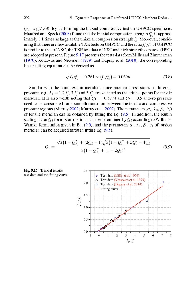
are adopted at present. Figure 9.17 presents the tests data from Mills and Zimmerman
(1970), Kotaovos and Newmen (1979) and Dupray et al. (2010), the corresponding
linear fitting equation can be derived as
J 2 /f
c = 0.261 ×
I 1 /f
c
+ 0.0396
(9.8)
Similar with the compression meridian, three another stress states at different
pressure, e.g., I 1 = 1.2 f
c , 3 f
c and 5 f
c , are selected as the critical points for tensile
meridian. It is also worth noting that Q 1 = 0.5774 and Q 2 = 0.5 at zero pressure
need to be considered for a smooth transition between the tensile and compressive
pressure regions (Murray 2007; Murray et al. 2007). The parameters (α 2 , λ 2 , β 2 , θ 2 )
of tensile meridian can be obtained by fitting the Eq. (9.5). In addition, the Rubin
scaling factor Q 1 for torsion meridian can be determined by Q 2 according to WilliansWarnke formulation given in Eq. (9.9), and the parameters α 1 , λ 1 , β 1 , θ 1 of torsion
meridian can be acquired through fitting Eq. (9.5).
Q 1 =
√
3
1 − Q
2
2
+ (2Q 2 − 1)
3
1 − Q
2
2
+ 5Q
2
2 − 4Q 2
3
1 − Q
2
2
+ (1 − 2Q 2 )
2
(9.9)
Fig. 9.17 Triaxial tensile
test data and the fitting curve
-1
0
1
2
3
4
5
6
7
8
0.0
0.5
1.0
1.5
2.0
2.5
1
c
I f
Test data (Mills et al. 1970)
Test data (Kotaovos et al. 1979)
Test data (Dupary et al. 2010)
Fitting curve
2
c
J f
9 Dynamic Responses of Reinforced UHPCC Members Under …
(σ 1 −σ 3 )/
√
3). By performing the biaxial compressive test on UHPCC specimens,
Manfred and Speck (2008) found that the biaxial compression strength f
bc is approximately 1.1 times as large as the uniaxial compression strength f
c . Moreover, considering that there are few available TXE tests on UHPCC and the ratio f
t /f
c of UHPCC
is similar to that of NSC, the TXE test data of NSC and high strength concrete (HSC)
are adopted at present. Figure 9.17 presents the tests data from Mills and Zimmerman
(1970), Kotaovos and Newmen (1979) and Dupray et al. (2010), the corresponding
linear fitting equation can be derived as
J 2 /f
c = 0.261 ×
I 1 /f
c
+ 0.0396
(9.8)
Similar with the compression meridian, three another stress states at different
pressure, e.g., I 1 = 1.2 f
c , 3 f
c and 5 f
c , are selected as the critical points for tensile
meridian. It is also worth noting that Q 1 = 0.5774 and Q 2 = 0.5 at zero pressure
need to be considered for a smooth transition between the tensile and compressive
pressure regions (Murray 2007; Murray et al. 2007). The parameters (α 2 , λ 2 , β 2 , θ 2 )
of tensile meridian can be obtained by fitting the Eq. (9.5). In addition, the Rubin
scaling factor Q 1 for torsion meridian can be determined by Q 2 according to WilliansWarnke formulation given in Eq. (9.9), and the parameters α 1 , λ 1 , β 1 , θ 1 of torsion
meridian can be acquired through fitting Eq. (9.5).
Q 1 =
√
3
1 − Q
2
2
+ (2Q 2 − 1)
3
1 − Q
2
2
+ 5Q
2
2 − 4Q 2
3
1 − Q
2
2
+ (1 − 2Q 2 )
2
(9.9)
Fig. 9.17 Triaxial tensile
test data and the fitting curve
-1
0
1
2
3
4
5
6
7
8
0.0
0.5
1.0
1.5
2.0
2.5
1
c
I f
Test data (Mills et al. 1970)
Test data (Kotaovos et al. 1979)
Test data (Dupary et al. 2010)
Fitting curve
2
c
J f