

9.4 Numerical Simulation
291
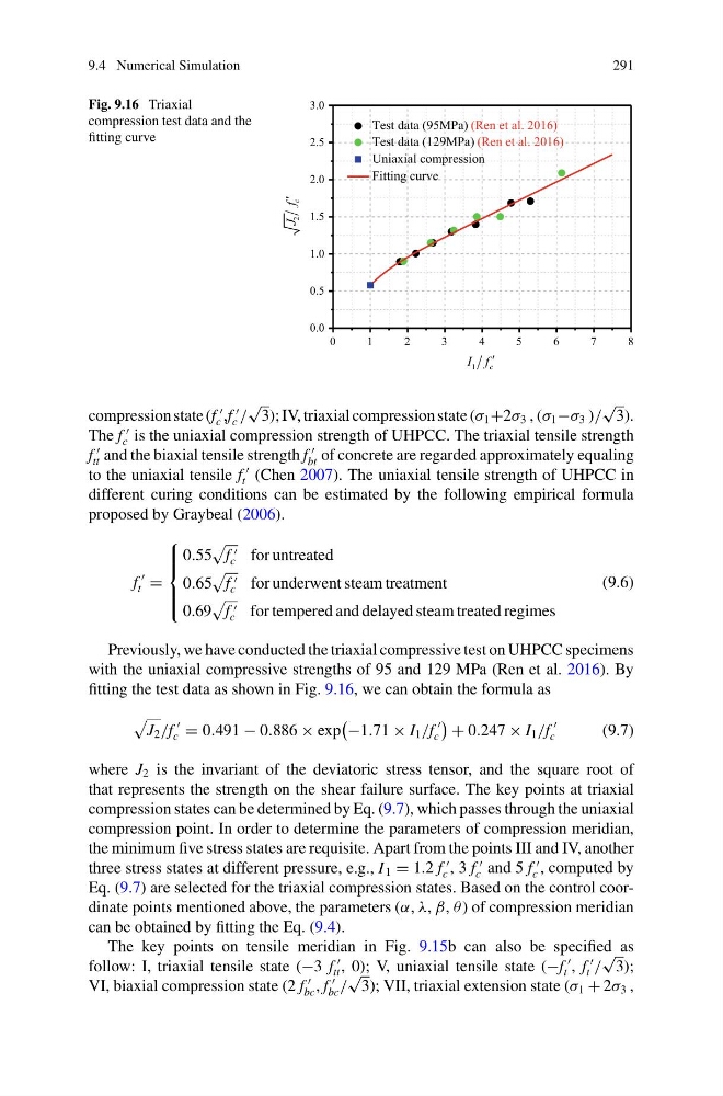
Fig. 9.16 Triaxial
compression test data and the
fitting curve
0
1
2
3
4
5
6
7
8
0.0
0.5
1.0
1.5
2.0
2.5
3.0
2
c
J f
Test data (95MPa) (Ren et al. 2016)
Test data (129MPa) (Ren et al. 2016)
Uniaxial compression
Fitting curve
1
c
I f
compression state (f
c ,f
c /
√
3); IV, triaxial compression state (σ 1 +2σ 3 , (σ 1 −σ 3 )/
√
3).
The f
c is the uniaxial compression strength of UHPCC. The triaxial tensile strength
f
tt and the biaxial tensile strength f
bt of concrete are regarded approximately equaling
to the uniaxial tensile f
t (Chen 2007). The uniaxial tensile strength of UHPCC in
different curing conditions can be estimated by the following empirical formula
proposed by Graybeal (2006).
f
t =
⎧
⎪ ⎪ ⎨
⎪ ⎪ ⎩
0.55
f
c for untreated
0.65
f
c for underwent steam treatment
0.69
f
c for tempered and delayed steam treated regimes
(9.6)
Previously, we have conducted the triaxial compressive test on UHPCC specimens
with the uniaxial compressive strengths of 95 and 129 MPa (Ren et al. 2016). By
fitting the test data as shown in Fig. 9.16, we can obtain the formula as
J 2 /f
c = 0.491 − 0.886 × exp
−1.71 × I 1 /f
c
+ 0.247 × I 1 /f
c
(9.7)
where J 2 is the invariant of the deviatoric stress tensor, and the square root of
that represents the strength on the shear failure surface. The key points at triaxial
compression states can be determined by Eq. (9.7), which passes through the uniaxial
compression point. In order to determine the parameters of compression meridian,
the minimum five stress states are requisite. Apart from the points III and IV, another
three stress states at different pressure, e.g., I 1 = 1.2 f
c , 3 f
c and 5 f
c , computed by
Eq. (9.7) are selected for the triaxial compression states. Based on the control coordinate points mentioned above, the parameters (α, λ, β, θ ) of compression meridian
can be obtained by fitting the Eq. (9.4).
The key points on tensile meridian in Fig. 9.15b can also be specified as
follow: I, triaxial tensile state (−3 f
tt , 0); V, uniaxial tensile state (−f
t , f
t /
√
3);
VI, biaxial compression state (2 f
bc , f
bc /
√
3); VII, triaxial extension state (σ 1 + 2σ 3 ,
291
Fig. 9.16 Triaxial
compression test data and the
fitting curve
0
1
2
3
4
5
6
7
8
0.0
0.5
1.0
1.5
2.0
2.5
3.0
2
c
J f
Test data (95MPa) (Ren et al. 2016)
Test data (129MPa) (Ren et al. 2016)
Uniaxial compression
Fitting curve
1
c
I f
compression state (f
c ,f
c /
√
3); IV, triaxial compression state (σ 1 +2σ 3 , (σ 1 −σ 3 )/
√
3).
The f
c is the uniaxial compression strength of UHPCC. The triaxial tensile strength
f
tt and the biaxial tensile strength f
bt of concrete are regarded approximately equaling
to the uniaxial tensile f
t (Chen 2007). The uniaxial tensile strength of UHPCC in
different curing conditions can be estimated by the following empirical formula
proposed by Graybeal (2006).
f
t =
⎧
⎪ ⎪ ⎨
⎪ ⎪ ⎩
0.55
f
c for untreated
0.65
f
c for underwent steam treatment
0.69
f
c for tempered and delayed steam treated regimes
(9.6)
Previously, we have conducted the triaxial compressive test on UHPCC specimens
with the uniaxial compressive strengths of 95 and 129 MPa (Ren et al. 2016). By
fitting the test data as shown in Fig. 9.16, we can obtain the formula as
J 2 /f
c = 0.491 − 0.886 × exp
−1.71 × I 1 /f
c
+ 0.247 × I 1 /f
c
(9.7)
where J 2 is the invariant of the deviatoric stress tensor, and the square root of
that represents the strength on the shear failure surface. The key points at triaxial
compression states can be determined by Eq. (9.7), which passes through the uniaxial
compression point. In order to determine the parameters of compression meridian,
the minimum five stress states are requisite. Apart from the points III and IV, another
three stress states at different pressure, e.g., I 1 = 1.2 f
c , 3 f
c and 5 f
c , computed by
Eq. (9.7) are selected for the triaxial compression states. Based on the control coordinate points mentioned above, the parameters (α, λ, β, θ ) of compression meridian
can be obtained by fitting the Eq. (9.4).
The key points on tensile meridian in Fig. 9.15b can also be specified as
follow: I, triaxial tensile state (−3 f
tt , 0); V, uniaxial tensile state (−f
t , f
t /
√
3);
VI, biaxial compression state (2 f
bc , f
bc /
√
3); VII, triaxial extension state (σ 1 + 2σ 3 ,