

142
5 Projectile Penetrations into Coarse Aggregated UHPCC Targets
o
A
D
C
B
x
y
Step 1
A
B
A
C
A
D
E
Step 2
A
B
A
C
A
D
E
F
Pn
Step 3
Step 4
(a)
(b)
(c)
(d)
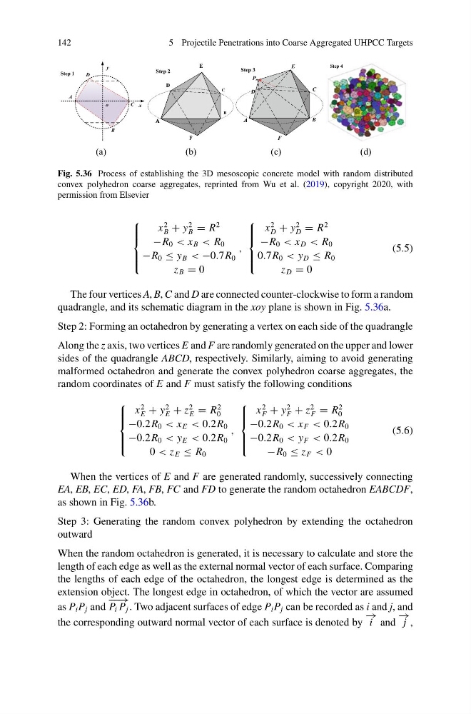
Fig. 5.36 Process of establishing the 3D mesoscopic concrete model with random distributed
convex polyhedron coarse aggregates, reprinted from Wu et al. (2019), copyright 2020, with
permission from Elsevier
⎧
⎪ ⎪ ⎨
⎪ ⎪ ⎩
x
2
B + y
2
B = R
2
−R 0 < x B < R 0
−R 0 ≤ y B < −0.7R 0
z B = 0
,
⎧
⎪ ⎪ ⎨
⎪ ⎪ ⎩
x
2
D + y
2
D = R
2
−R 0 < x D < R 0
0.7R 0 < y D ≤ R 0
z D = 0
(5.5)
The four vertices A, B, C and D are connected counter-clockwise to form a random
quadrangle, and its schematic diagram in the xoy plane is shown in Fig. 5.36a.
Step 2: Forming an octahedron by generating a vertex on each side of the quadrangle
Along the z axis, two vertices E and F are randomly generated on the upper and lower
sides of the quadrangle ABCD, respectively. Similarly, aiming to avoid generating
malformed octahedron and generate the convex polyhedron coarse aggregates, the
random coordinates of E and F must satisfy the following conditions
⎧
⎪ ⎪ ⎨
⎪ ⎪ ⎩
x
2
E + y
2
E + z
2
E = R
2
0
−0.2R 0 < x E < 0.2R 0
−0.2R 0 < y E < 0.2R 0
0 < z E ≤ R 0
,
⎧
⎪ ⎪ ⎨
⎪ ⎪ ⎩
x
2
F + y
2
F + z
2
F = R
2
0
−0.2R 0 < x F < 0.2R 0
−0.2R 0 < y F < 0.2R 0
−R 0 ≤ z F < 0
(5.6)
When the vertices of E and F are generated randomly, successively connecting
EA, EB, EC, ED, FA, FB, FC and FD to generate the random octahedron EABCDF,
as shown in Fig. 5.36b.
Step 3: Generating the random convex polyhedron by extending the octahedron
outward
When the random octahedron is generated, it is necessary to calculate and store the
length of each edge as well as the external normal vector of each surface. Comparing
the lengths of each edge of the octahedron, the longest edge is determined as the
extension object. The longest edge in octahedron, of which the vector are assumed
as P i P j and
− − →
P i P j . Two adjacent surfaces of edge P i P j can be recorded as i and j, and
the corresponding outward normal vector of each surface is denoted by
− →
i and
− →
j ,
5 Projectile Penetrations into Coarse Aggregated UHPCC Targets
o
A
D
C
B
x
y
Step 1
A
B
A
C
A
D
E
Step 2
A
B
A
C
A
D
E
F
Pn
Step 3
Step 4
(a)
(b)
(c)
(d)
Fig. 5.36 Process of establishing the 3D mesoscopic concrete model with random distributed
convex polyhedron coarse aggregates, reprinted from Wu et al. (2019), copyright 2020, with
permission from Elsevier
⎧
⎪ ⎪ ⎨
⎪ ⎪ ⎩
x
2
B + y
2
B = R
2
−R 0 < x B < R 0
−R 0 ≤ y B < −0.7R 0
z B = 0
,
⎧
⎪ ⎪ ⎨
⎪ ⎪ ⎩
x
2
D + y
2
D = R
2
−R 0 < x D < R 0
0.7R 0 < y D ≤ R 0
z D = 0
(5.5)
The four vertices A, B, C and D are connected counter-clockwise to form a random
quadrangle, and its schematic diagram in the xoy plane is shown in Fig. 5.36a.
Step 2: Forming an octahedron by generating a vertex on each side of the quadrangle
Along the z axis, two vertices E and F are randomly generated on the upper and lower
sides of the quadrangle ABCD, respectively. Similarly, aiming to avoid generating
malformed octahedron and generate the convex polyhedron coarse aggregates, the
random coordinates of E and F must satisfy the following conditions
⎧
⎪ ⎪ ⎨
⎪ ⎪ ⎩
x
2
E + y
2
E + z
2
E = R
2
0
−0.2R 0 < x E < 0.2R 0
−0.2R 0 < y E < 0.2R 0
0 < z E ≤ R 0
,
⎧
⎪ ⎪ ⎨
⎪ ⎪ ⎩
x
2
F + y
2
F + z
2
F = R
2
0
−0.2R 0 < x F < 0.2R 0
−0.2R 0 < y F < 0.2R 0
−R 0 ≤ z F < 0
(5.6)
When the vertices of E and F are generated randomly, successively connecting
EA, EB, EC, ED, FA, FB, FC and FD to generate the random octahedron EABCDF,
as shown in Fig. 5.36b.
Step 3: Generating the random convex polyhedron by extending the octahedron
outward
When the random octahedron is generated, it is necessary to calculate and store the
length of each edge as well as the external normal vector of each surface. Comparing
the lengths of each edge of the octahedron, the longest edge is determined as the
extension object. The longest edge in octahedron, of which the vector are assumed
as P i P j and
− − →
P i P j . Two adjacent surfaces of edge P i P j can be recorded as i and j, and
the corresponding outward normal vector of each surface is denoted by
− →
i and
− →
j ,